8 辅助工具使用教程

备注

用DSPAW完成DFT计算后，想快速分析结果、画图，或者完成一些常见的数据处理任务？

dspawpy （ Python ≥ 3.9 ）就是这样一款辅助工具，它可以编程调用（参考下文示例脚本），也提供了一个命令行交互程序

参考下方教程安装后，命令行输入 dspawpy 后回车即可使用交互程序：

 ... loading dspawpy cli ...

 ********这是dspawpy命令行交互小工具，预祝您使用愉快********
    ( )
   _| |  ___  _ _      _ _  _   _   _  _ _    _   _
 /'_` |/',__)( '_`\  /'_` )( ) ( ) ( )( '_`\ ( ) ( )
( (_| |\__, \| (_) )( (_| || \_/ \_/ || (_) )| (_) |
 \__,_)(____/| ,__/'`\__,_) \___x___/ | ,__/  \__, |
             | |                      | |    ( )_| |
             (_)                      (_)     \___/

 [版本号]: [安装路径]

 ======================================
 |  1: update更新
 |  2: structure结构转化
 |  3: volumetricData数据处理
 |  4: band能带数据处理
 |  5: dos态密度数据处理
 |  6: bandDos能带和态密度共同显示
 |  7: optical光学性质数据处理
 |  8: neb过渡态计算数据处理
 |  9: phonon声子计算数据处理
 |  10: aimd分子动力学模拟数据处理
 |  11: Polarization铁电极化数据处理
 |  12: ZPE零点振动能数据处理
 |  13: TS的热校正能
 |
 |  q: 退出
 ======================================
 --> 输入数字后回车选择功能：

亮点：

自动补全：按Tab键即可生效，有助于快速且正确地输入程序所需要的参数
多线程懒加载：在等待用户输入时后台加载模块，大幅缩短等待时间；仅加载必要模块，减少内存占用

注意：

在远程服务器上使用时，由于机器的磁盘读写性能不佳，可能需要较长的启动时间，极端情况下可能长达半分钟（与服务器当时的磁盘读写性能直接相关）。如果无法忍受，请在自己的电脑上安装dspawpy使用
输入 dspawpy 回车后，python会先加载内建模块，完成后显示 ... loading dspawpy cli ... 提示语句，表明进入第二阶段（开始加载第三方依赖库）
等待第二阶段完成后，会显示欢迎界面，此时dspwapy已完成前期加载，进入第三阶段。后续将动态根据选择的功能模块加载相应的依赖库，从而最大限度减少等待时间

8.1 安装与更新

在HZW机器上，已提前安装 dspawpy，使用以下命令激活虚拟环境即可使用：

source /data/hzwtech/profile/dspawpy.env

在其他机器上，请自行安装 dspawpy（下列两种方式二选一）：

使用 mamba 或 conda ，安装包可前往 https://conda-forge.org/download/ 下载

mamba install dspawpy -c conda-forge
#conda install dspawpy -c conda-forge

或使用 pip3 (部分操作系统中没有pip3可执行程序，此时请尝试pip)

pip3 install dspawpy

关于如何设置pip和conda镜像地址以加速安装过程，可参考 https://mirrors.tuna.tsinghua.edu.cn/help/pypi/ 和 https://mirrors.tuna.tsinghua.edu.cn/help/anaconda/

如果安装依然失败，请尝试上面的 mamba/conda 安装法。

警告

在集群上，由于权限问题，公共路径中的pip很可能不支持全局安装python库，必须在 pip install 后面追加 --user 选项安装到家目录 ~/.local/lib/python3.x/site-packages/ 下，其中3.x表示python解释器版本，x可能是9-13之间的任意整数

python将优先读取家目录下的dspawpy，即使公共环境中的dspawpy的版本比家目录中的dspawpy的版本新! 因此，如果以前用 --user 安装过dspawpy，又忘记手动更新家目录下的老版本dspawpy，即使source了公共环境，也无法调用公共环境中的dspawpy，依旧会使用老版本dspawpy，导致一些BUG。

因此，鉴于HZW集群每周自动更新dspawpy，建议不要在家目录下重复安装，已安装的建议删除 。如果在其他集群上，请确保及时手动更新家目录下的 dspawpy

如果不想删除家目录中的dspawpy，又不想更新它，可以在运行python脚本时，尝试 -s 选项避免导入家目录中的 dspawpy： python -s your-script.py。

更新 dspawpy

如果 dspawpy 是通过 mamba/conda 安装的，使用以下命令更新：

mamba update dspawpy
#conda update dspawpy

如果 dspawpy 是通过 pip 安装的，那么：

pip install dspawpy -U # -U 表示安装最新版

备注

如果 pip 使用了国内的镜像网站，可能由于镜像网站尚未同步最新版 dspawpy 而导致无法顺利升级，请使用如下命令告诉 pip 从pypi官网下载安装：

pip install dspawpy -i https://pypi.org/simple --user -U # -i 指定下载地址，--user 表示仅为当前用户安装，-U 表示安装最新版

如果运行时出现 dspawpy 相关 错误信息，请先检查是否已正确导入最新版本的 dspawpy 并检查安装路径：

$ python3 # 或 python
>>> import dspawpy
>>> dspawpy.__version__ # 将输出版本号
>>> dspawpy.__file__ # 将输出安装路径

8.2 structure结构转化

读取结构信息使用 read 函数；将结构信息写入文件，使用 write 函数；快速结构转化，使用 convert 函数：

可参考 2conversion.py 脚本完成转化：

# coding:utf-8
from dspawpy.io.structure import convert

convert(
    infile="dspawpy_proj/dspawpy_tests/inputs/2.1/relax.h5",  # Structure to be converted, if in the current path, you can just write the filename
    si=None,  # Select configuration number, if not specified, read all by default
    ele=None,  # Filter element symbol, default reads atomic information for all elements
    ai=None,  # Filter atomic indices, starting from 1, default to read all atomic information
    infmt=None,  # Input structure file type, e.g., 'h5'. If None, it will be matched ambiguously based on the filename rule.
    task="relax",  # Task type, this parameter is only valid when infile is a folder rather than a filename
    outfile="dspawpy_proj/dspawpy_tests/outputs/us/relaxed.xyz",  # Structure file name
    outfmt=None,  # Output structure file type, e.g., 'xyz'. If None, it will be fuzzy matched according to filename rules.
    coords_are_cartesian=True,  # Written in Cartesian coordinates by default
)

convert 函数的几个关键参数设置规则见下表：

**dspawpy 支持读写的结构文件列表**
infmt（输入文件格式）	infile（输入文件名模糊匹配）	outfmt（输出文件格式）	outfile（输出文件名模糊匹配）	说明
h5	*.h5	X	X	DS-PAW计算完成后保存的hdf5类型文件
json	*.json	json	*.json	DS-PAW计算完成后保存的json类型文件
pdb	*.pdb	pdb	*.pdb	Protein Data Bank
as	*.as	as	*.as	DS-PAW记载原子坐标等信息的结构文件
hzw	*.hzw	hzw	*.hzw	DeviceStudio默认的结构文件
xyz	*.xyz	xyz	*.xyz	读取时仅支持分子结构的单构型，写入时则是包含晶胞的extended-xyz类型轨迹文件
X	X	dump	*.dump	lammps-dump类型轨迹文件
X	.cif/.mcif	cif/mcif	.cif/.mcif	Crystallographic Information File
X	POSCAR/CONTCAR/.vasp/CHGCAR/LOCPOT/vasprun.xml*	poscar	POSCAR	VASP文件
X	.cssr	cssr	.cssr	Crystal Structure Standard Representation
X	.yaml/.yml	yaml/yml	.yaml/.yml	YAML Ain't Markup Language
X	.xsf	xsf	.xsf	eXtended Structural Format
X	rndstr.in/lat.in/bestsqs	mcsqs	rndstr.in/lat.in/bestsqs	Monte Carlo Special Quasirandom Structure
X	inp.xml/.in/inp_	fleur-inpgen	.in	FLEUR 结构文件，须额外安装 pymatgen-io-fleur 库
X	*.res	res	*.res	ShelX res 结构文件
X	.config/.pwmat	pwmat	.config/.pwmat	PWmat 文件
X	X	prismatic	prismatic	用于STEM模拟的一种文件格式
X	CTRL*	X	X	Stuttgart LMTO-ASA 文件

备注

上述表格中 * 号表示任意字符，X 表示不支持
h5, json, pdb, xyz, dump, CONTCAR等格式支持多个结构组成的轨迹信息（常见于结构优化或者NEB或者AIMD任务）
in(out)fmt 参数优先级高于文件名模糊匹配规则；例如，指定 in(out)fmt='h5' 后，文件名可以是任意值，甚至可以是 a.json
将结构信息写为 json 格式时，仅支持可视化 NEB 链任务，详见观察NEB链节相关说明
DS-PAW 输出的 neb.h5、phonon.h5、phonon.json、neb.json以及wannier.json 暂时无法读取结构信息

8.3 volumetricData数据处理

volumetricData可视化

参考 3vis_vol.py ：

# coding:utf-8
from dspawpy.io.write import write_VESTA

# Read data file (in h5 or json format), process it, and output to a cube file
write_VESTA(
    in_filename="dspawpy_proj/dspawpy_tests/inputs/2.2/rho.h5",  # Path to the json or h5 file containing electronic system information
    data_type="rho",  # Data type, supported values are "rho", "potential", "elf", "pcharge", "rhoBound"
    out_filename="dspawpy_proj/dspawpy_tests/outputs/us/DS-PAW_rho.cube",  # Output file path
    gridsize=(10, 10, 10),  # Specifies the interpolation grid size
    format="cube",  # Supported formats: cube, vesta, and txt (xyz grid coordinates + values)
)

将转换后的文件 DS-PAW_rho.cube 拖入 VESTA 软件中显示：

晶体硅单胞的电荷密度分布示意图

差分volumetricData可视化

参考 3dvol.py ：

# coding:utf-8
from dspawpy.io.write import write_delta_rho_vesta

# Read the data file (h5 or json format), process it, and output it to a cube file, which can be directly opened with Vesta and has a small volume
write_delta_rho_vesta(
    total="dspawpy_proj/dspawpy_tests/inputs/supplement/AB.h5",  # Data file for the system containing all components
    individuals=[
        "dspawpy_proj/dspawpy_tests/inputs/supplement/A.h5",
        "dspawpy_proj/dspawpy_tests/inputs/supplement/B.h5",
    ],  # Data files for the system containing each component
    output="dspawpy_proj/dspawpy_tests/outputs/us/3delta_rho.cube",  # Output file path
)

上述脚本支持处理多元体系的电荷密度差，示例以二元体系为例，得到了 AB.h5 与 A.h5 和 B.h5 之间的电荷密度差文件 delta_rho.cube ，该文件可直接使用 VESTA 打开。

volumetricData面平均

参考 3planar_ave.py ：

# coding:utf-8
from dspawpy.plot import average_along_axis

axes = [
    "2"
]  # "0", "1", "2" correspond to the x, y, z axes respectively; select which axes to average along
axes_indices = [int(i) for i in axes]
for ai in axes_indices:
    plt = average_along_axis(
        datafile="dspawpy_proj/dspawpy_tests/inputs/3.3/scf.h5",  # Data file path
        task="potential",  # Task name, can be 'rho', 'potential', 'elf', 'pcharge', 'rhoBound'
        axis=ai,  # Axis along which to plot the potential curve
        smooth=False,  # Whether to smooth
        smooth_frac=0.8,  # Smoothing coefficient
        subtype=None,  # Used to specify the subclass of task data, currently only used for Potential
        label=f"axis{ai}",  # Legend label
    )
if len(axes_indices) > 1:
    plt.legend()

plt.xlabel("Grid Index")
plt.ylabel("TotalElectrostaticPotential (eV)")
plt.savefig("dspawpy_proj/dspawpy_tests/outputs/us/3pot_ave.png", dpi=300)  # Image name

处理应用案例 3.3 小节所得静电势文件，可得真空方向势函数曲线如下所示：

AuAl势函数示意图

警告

如果通过SSH连接到远程服务器执行上述脚本，出现QT相关的报错信息，可能是使用的程序（比如MobaXterm等）和QT库不兼容，要么更换程序（例如VSCode或者系统自带的终端命令行），要么请在python脚本第二行开始添加以下代码：

import matplotlib
matplotlib.use('agg')

8.4 band能带数据处理

知识点：

脚本中调用get_band_data()读取数据，在读取数据时设置efermi=XX可将能量零点修改为指定值；设置zero_to_efermi=True, 可将能量零点修改问所读取的文件中的费米能级处
脚本调用pymatgen的BSPlotter.get_plot()画图，在画图时可设置zero_to_efermi=True，将坐标轴能量零点修改到费米能级处。由于pymatgen在2023.8.17的一处关键更新将绘图函数返回对象从plt改成了axes，导致后续脚本可能出现不兼容。因此用户脚本相关部分已添加一个判断语句加以处理。
能带两步算需从第一步自洽计算获取准确费米能级（从自洽获得的system.json），若获取失败，用户可在调用get_band_data读取数据时，利用参数efermi修改能量零点。例如：band_data=get_band_data('band.h5',efermi=-1.5)
脚本中画图调用pymatgen中的BSPlotter.get_plot, 当判断体系为非金属时，设置zero_to_efermi会认为VBM为费米能级能量而非文件读取时的费米能级。故当体系为非金属时，在数据读取时设置zero_to_efermi=True和在画图时设置zero_to_efermi=True得到的图会有区别

执行本节所列的python脚本，程序会判断是否为金属体系。若为非金属体系，将要求选择是否平移费米能级到能量零点，请按提示操作。

如有必要，参考 export_band.py 将能带数据提取出来并写入csv文件：

# coding:utf-8
from dspawpy.io.export import read_band

band_data = read_band(
    bandfile="dspawpy_proj/dspawpy_tests/inputs/2.4/band.h5",
    mode=1,  # projection mode, only valid for pband data
    hide_index=False,  # hide index column or not
    fmt="8.3f",  # decimal format to print
)
band_data.write_csv("banddata.csv")

投影模式 mode 可以设置成 1~5 ，分别对应

元素
元素 + spdf 轨道
元素 + spxpypz... 轨道
原子 + spdf 轨道
原子 + spxpypz... 轨道

其中，4、5两种投影模式输出的数据表格中，第一个数字表示能带编号，第二个数字表示原子编号，都从 1 开始；比如 2-1-s 表示第二条能带中第一个原子的s轨道贡献

API: read_band()

dspawpy.io.export.read_band(bandfile: str | Path, mode: int = 5, hide_index: bool = False, fmt: str = '8.3f')

Construct a dataframe of band structure data from an h5 or json file.

参数:

bandfile (str | Path) -- band data file location, such as 'band.json'.
mode (int) -- which projection mode, only valid for pband data.
hide_index (bool) -- hide index column in dataframe or not.
fmt (str) -- control display decimal, such as '8.3f'

示例

>>> from dspawpy.io.export import read_band
>>> read_band(bandfile='dspawpy_proj/dspawpy_tests/inputs/2.3/band.h5')
efermi=5.1696 eV
shape: (150, 16)
┌───────┬──────────┬──────────┬──────────┬───┬──────────┬──────────┬──────────┬──────────┐
│ index ┆ kx       ┆ ky       ┆ kz       ┆ … ┆ 9        ┆ 10       ┆ 11       ┆ 12       │
╞═══════╪══════════╪══════════╪══════════╪═══╪══════════╪══════════╪══════════╪══════════╡
│ 1     ┆    0.000 ┆    0.500 ┆    0.246 ┆ … ┆   -4.950 ┆    7.858 ┆   -6.766 ┆    8.395 │
│ 2     ┆    0.000 ┆    0.172 ┆    0.246 ┆ … ┆   -0.491 ┆    9.558 ┆    3.944 ┆   12.139 │
│ 3     ┆    0.000 ┆    0.672 ┆    0.491 ┆ … ┆    1.294 ┆   11.707 ┆    4.708 ┆   12.457 │
│ 4     ┆    0.017 ┆    0.500 ┆    0.233 ┆ … ┆    3.604 ┆   12.532 ┆    4.708 ┆   12.457 │
│ 5     ┆    0.000 ┆    0.181 ┆    0.233 ┆ … ┆    7.334 ┆   13.710 ┆    7.369 ┆   13.616 │
│ …     ┆ …        ┆ …        ┆ …        ┆ … ┆ …        ┆ …        ┆ …        ┆ …        │
│ 146   ┆    0.155 ┆    0.272 ┆    0.483 ┆ … ┆    3.067 ┆    8.304 ┆    0.255 ┆   12.534 │
│ 147   ┆    0.655 ┆    0.543 ┆    0.483 ┆ … ┆    3.906 ┆   12.505 ┆    3.982 ┆   15.529 │
│ 148   ┆    0.500 ┆    0.259 ┆    0.500 ┆ … ┆    4.713 ┆   12.505 ┆    3.982 ┆   15.942 │
│ 149   ┆    0.164 ┆    0.259 ┆    0.500 ┆ … ┆    7.675 ┆   12.908 ┆    6.606 ┆   16.040 │
│ 150   ┆    0.664 ┆    0.517 ┆    0.500 ┆ … ┆    7.700 ┆   16.401 ┆    8.395 ┆   17.259 │
└───────┴──────────┴──────────┴──────────┴───┴──────────┴──────────┴──────────┴──────────┘

普通能带处理

参考 4bandplot.py ：

# coding:utf-8
import os
import matplotlib.pyplot as plt
from pymatgen.electronic_structure.plotter import BSPlotter

from dspawpy.io.read import get_band_data

datafile = "dspawpy_proj/dspawpy_tests/inputs/supplement/pband.h5"  # Specifies the data file path
band_data = get_band_data(
    band_dir=datafile,
    syst_dir=None,  # path to system.json file, required only when band_dir is a json file
    efermi=None,  # Used for manually correcting the Fermi level
    zero_to_efermi=True,  # For non-metallic systems, the zero point energy should be shifted to the Fermi level
)

bsp = BSPlotter(band_data)
axes_or_plt = bsp.get_plot(
    zero_to_efermi=False,  # The data has already been shifted when read, so this should be turned off
    ylim=[-10, 10],  # Range of the y-axis for the band structure plot
    smooth=False,  # Whether to smooth the band structure plot
    vbm_cbm_marker=False,  # Whether to mark the valence band maximum and conduction band minimum in the band structure plot
    smooth_tol=0,  # Threshold for smoothing
    smooth_k=3,  # Order of the smoothing process
    smooth_np=100,  # Number of points for smoothing
)

if isinstance(axes_or_plt, plt.Axes):
    fig = axes_or_plt.get_figure()  # version newer than v2023.8.10
else:
    fig = axes_or_plt.gcf()  # older version pymatgen

# Add a reference line for the energy zero point
for ax in fig.axes:
    ax.axhline(0, lw=2, ls="-.", color="gray")

figname = "dspawpy_proj/dspawpy_tests/outputs/us/4bandplot.png"  # Filename for the output band plot
os.makedirs(os.path.dirname(os.path.abspath(figname)), exist_ok=True)
fig.savefig(figname, dpi=300)

知识点：

能带两步算需从自洽计算获取准确的费米能级（从system.json获取），若获取失败，用户可在 get_band_data 函数中指定 efermi 参数修改

执行代码可以得到类似以下能带图：

二硫化钼能带示意图

将能带投影到每一种元素分别作图，数据点大小表示该元素对该轨道的贡献

参考 4bandplot_elt.py ：

# coding:utf-8
import os

import matplotlib.pyplot as plt
import numpy as np
from pymatgen.electronic_structure.plotter import BSPlotterProjected

from dspawpy.io.read import get_band_data

datafile = "dspawpy_proj/dspawpy_tests/inputs/supplement/pband.h5"  # Specify the data file path
band_data = get_band_data(
    band_dir=datafile,
    syst_dir=None,  # path to system.json file, required only when band_dir is a json file
    efermi=None,  # Used to manually adjust the Fermi level
    zero_to_efermi=True,  # For non-metallic systems, shift the zero-point energy to the Fermi level
)

bsp = BSPlotterProjected(bs=band_data)  # Initialize the BSPlotterProjected class
axes_or_plt = bsp.get_elt_projected_plots(
    zero_to_efermi=False,  # The data has already been shifted when read, so this should be disabled
    ylim=[-8, 5],  # Set the energy range
    vbm_cbm_marker=False,  # Whether to mark the conduction band minimum (CBM) and valence band maximum (VBM)
)

if isinstance(axes_or_plt, plt.Axes):
    fig = axes_or_plt.get_figure()  # version newer than v2023.8.10
elif np.iterable(axes_or_plt):
    fig = np.asarray(axes_or_plt).flatten()[0].get_figure()
else:
    fig = axes_or_plt.gcf()  # older version pymatgen

# Add a reference line for the energy zero point
for ax in fig.axes:
    ax.axhline(0, lw=2, ls="-.", color="gray")

figname = "dspawpy_proj/dspawpy_tests/outputs/us/4bandplot_elt.png"  # The filename for the output band plot
os.makedirs(os.path.dirname(os.path.abspath(figname)), exist_ok=True)
fig.savefig(figname, dpi=300)

知识点：

用户如果需要绘制能带投影的数据，此时需要使用 BSPlotterProjected模块
使用 BSPlotterProjected模块中 get_elt_projected_plots 函数能够绘制每种元素对轨道贡献的能带图

执行代码可以得到类似以下能带图：

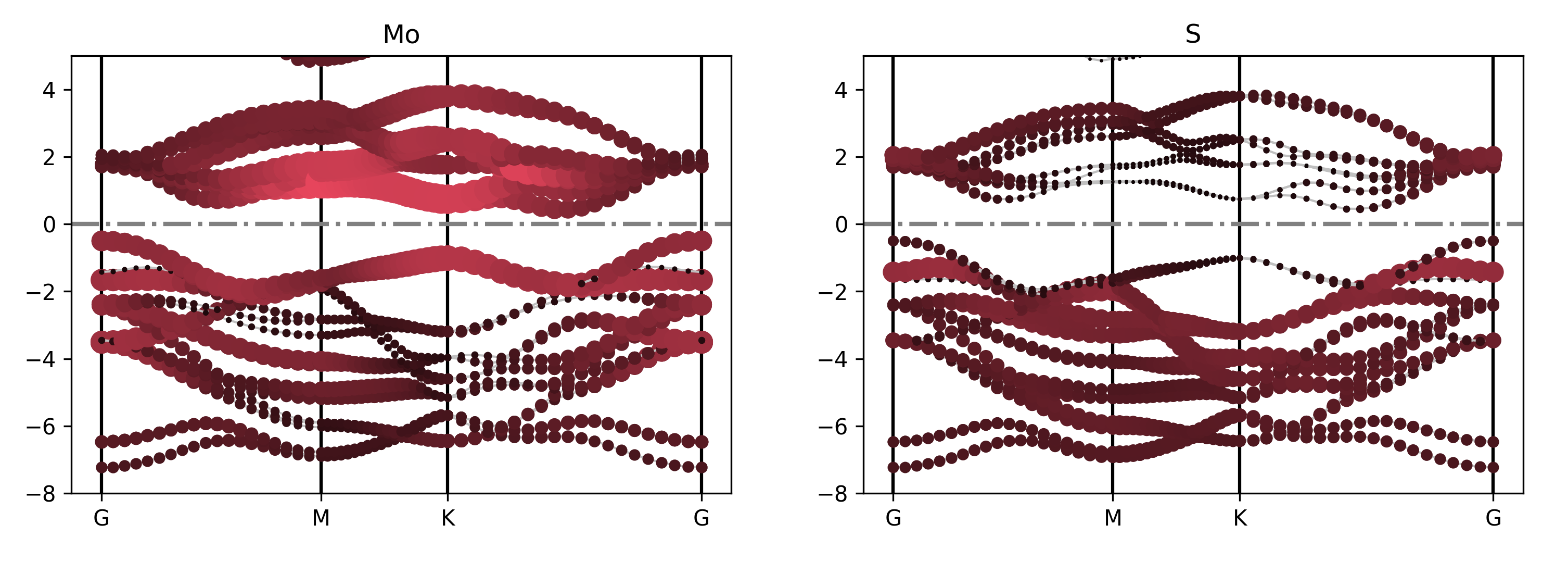
二硫化钼元素投影能带示意图

警告

如果通过SSH连接到远程服务器执行上述脚本，出现QT相关的报错信息，可能是使用的程序（比如MobaXterm等）和QT库不兼容，要么更换程序（例如VSCode或者系统自带的终端命令行），要么请在python脚本第二行开始添加以下代码：

import matplotlib
matplotlib.use('agg')

能带投影到不同元素的不同轨道

参考 4bandplot_elt_orbit.py ：

# coding:utf-8
import os

import matplotlib.pyplot as plt
import numpy as np
from pymatgen.electronic_structure.plotter import BSPlotterProjected

from dspawpy.io.read import get_band_data

datafile = "dspawpy_proj/dspawpy_tests/inputs/supplement/pband.h5"  # Specify the data file path
band_data = get_band_data(
    band_dir=datafile,
    syst_dir=None,  # path to system.json file, only required when band_dir is a json file
    efermi=None,  # Used for manually correcting the Fermi level
    zero_to_efermi=True,  # For non-metallic systems, shift the zero point energy to the Fermi level
)

bsp = BSPlotterProjected(bs=band_data)  # Initialize the BSPlotterProjected class
# Select elements and orbitals, create a dictionary
dict_elem_orbit = {"Mo": ["d"], "S": ["s"]}

axes_or_plt = bsp.get_projected_plots_dots(
    dictio=dict_elem_orbit,
    zero_to_efermi=False,  # The data has already been shifted when read, so this should be turned off
    ylim=[-8, 5],  # Set the energy range
    vbm_cbm_marker=False,  # Whether to mark the conduction band minimum and valence band maximum
)

if isinstance(axes_or_plt, plt.Axes):
    fig = axes_or_plt.get_figure()  # version newer than v2023.8.10
elif np.iterable(axes_or_plt):
    fig = np.asarray(axes_or_plt).flatten()[0].get_figure()
else:
    fig = axes_or_plt.gcf()  # older version pymatgen

# Add a reference line for the energy zero point
for ax in fig.axes:
    ax.axhline(0, lw=2, ls="-.", color="gray")

figname = "dspawpy_proj/dspawpy_tests/outputs/us/4bandplot_elt_orbit.png"  # Filename for the output band plot
os.makedirs(os.path.dirname(os.path.abspath(figname)), exist_ok=True)
fig.savefig(figname, dpi=300)

知识点：

使用 BSPlotterProjected模块中 get_projected_plots_dots可以让用户来自定义需要绘制的某种元素某种轨道(L)的能带图
例如 get_projected_plots_dots ({'Mo':['d'],'S':['s']})就是绘制Mo的d轨道和S的s轨道

执行代码可以得到类似以下能带图：

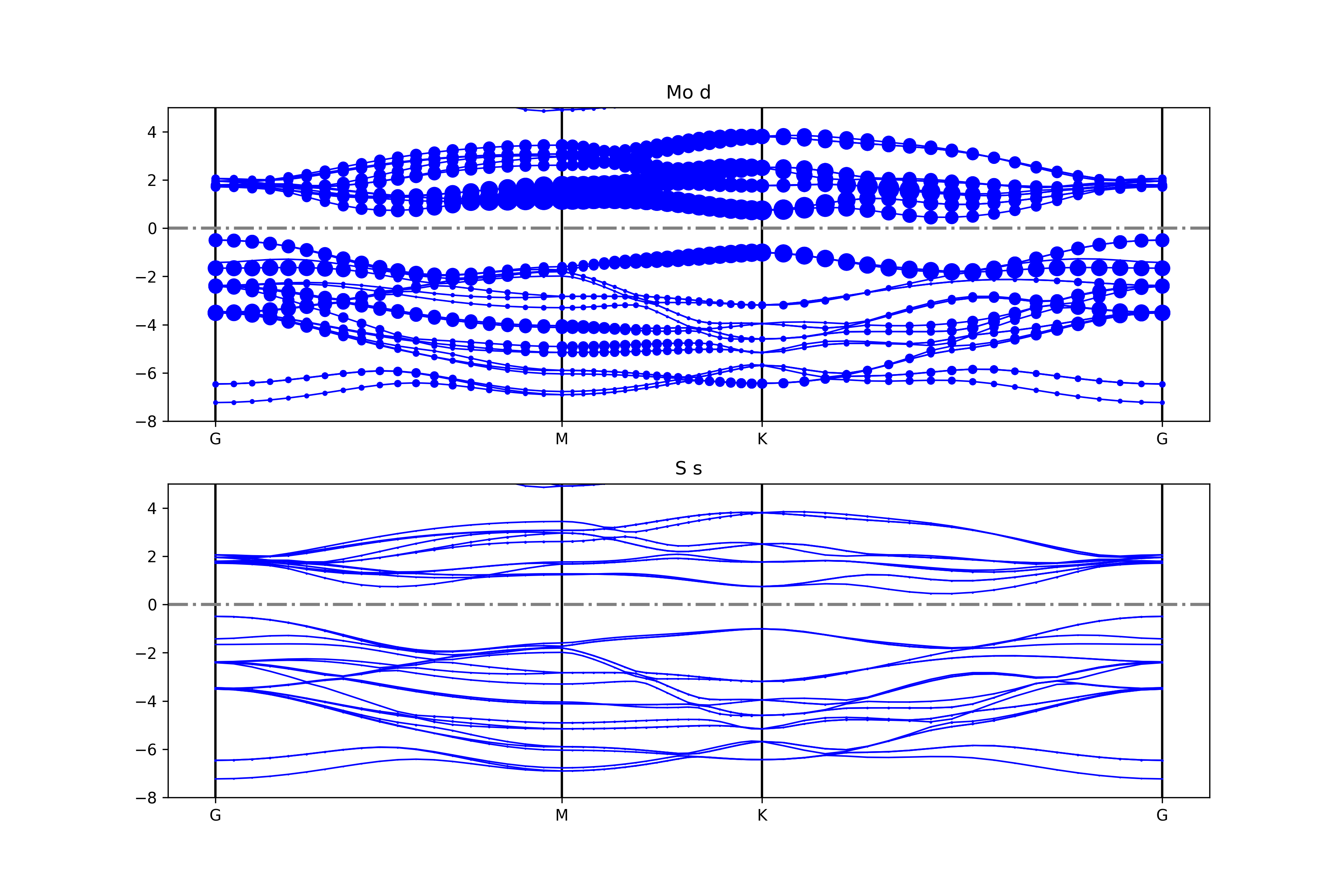
二硫化钼元素轨道投影能带示意图

警告

如果通过SSH连接到远程服务器执行上述脚本，出现QT相关的报错信息，可能是使用的程序（比如MobaXterm等）和QT库不兼容，要么更换程序（例如VSCode或者系统自带的终端命令行），要么请在python脚本第二行开始添加以下代码：

import matplotlib
matplotlib.use('agg')

将能带投影到不同原子的不同轨道

参考 4bandplot_patom_porbit.py ：

# coding:utf-8
import os

import matplotlib.pyplot as plt
import numpy as np
from pymatgen.electronic_structure.plotter import BSPlotterProjected

from dspawpy.io.read import get_band_data

datafile = "dspawpy_proj/dspawpy_tests/inputs/supplement/pband.h5"  # Specify the data file path
band_data = get_band_data(
    band_dir=datafile,
    syst_dir=None,  # path to system.json file, required only when band_dir is a JSON file
    efermi=None,  # Used to manually adjust the Fermi level
    zero_to_efermi=True,  # For non-metallic systems, shift the zero point energy to the Fermi level
)

bsp = BSPlotterProjected(bs=band_data)
# Specify elements, orbitals, and atomic numbers
dict_elem_orbit = {"Mo": ["px", "py", "pz"]}
dict_elem_index = {"Mo": [1]}

axes_or_plt = bsp.get_projected_plots_dots_patom_pmorb(
    dictio=dict_elem_orbit,  # Specify the element-orbit dictionary
    dictpa=dict_elem_index,  # Specify the element-atomic number dictionary
    sum_atoms=None,  # Whether to sum over atoms
    sum_morbs=None,  # Whether to sum orbitals
    zero_to_efermi=False,  # Data has already been shifted during reading, should be turned off here
    ylim=None,  # Set the energy range
    vbm_cbm_marker=False,  # Whether to mark the conduction band minimum and valence band maximum
    selected_branches=None,  # Specify the energy band branches to be plotted
    w_h_size=(12, 8),  # Set image width and height
    num_column=None,  # Number of images displayed per row
)

if isinstance(axes_or_plt, plt.Axes):
    fig = axes_or_plt.get_figure()  # version newer than v2023.8.10
elif np.iterable(axes_or_plt):
    fig = np.asarray(axes_or_plt).flatten()[0].get_figure()
else:
    fig = axes_or_plt.gcf()  # older version pymatgen

# Add a reference line for the energy zero point
for ax in fig.axes:
    ax.axhline(0, lw=2, ls="-.", color="gray")

figname = " dspawpy_proj/dspawpy_tests/outputs/us/4band_patom_porbit.png"  # Output bandpass figure filename
os.makedirs(os.path.dirname(os.path.abspath(figname)), exist_ok=True)
fig.savefig(figname, dpi=300)

知识点：

使用 BSPlotterProjected模块中 get_projected_plots_dots_patom_pmorb 的自由度更高，可以让用户来自定义需要绘制的某些原子某些轨道的能带图
dictpa指定原子，dictio 指定该原子的轨道
如果要将一些原子或一些轨道的投影分量叠加起来，请根据 get_projected_plots_dots_patom_pmorb 函数文档指定 sum_atoms 或 sum_morbs 参数

警告

如果只选择单个轨道，且轨道名称不止一个字母（例如px、dxy、dxz），get_projected_plots_dots_patom_pmorb 函数将报错，详情见此处

执行代码可以得到类似以下能带图：

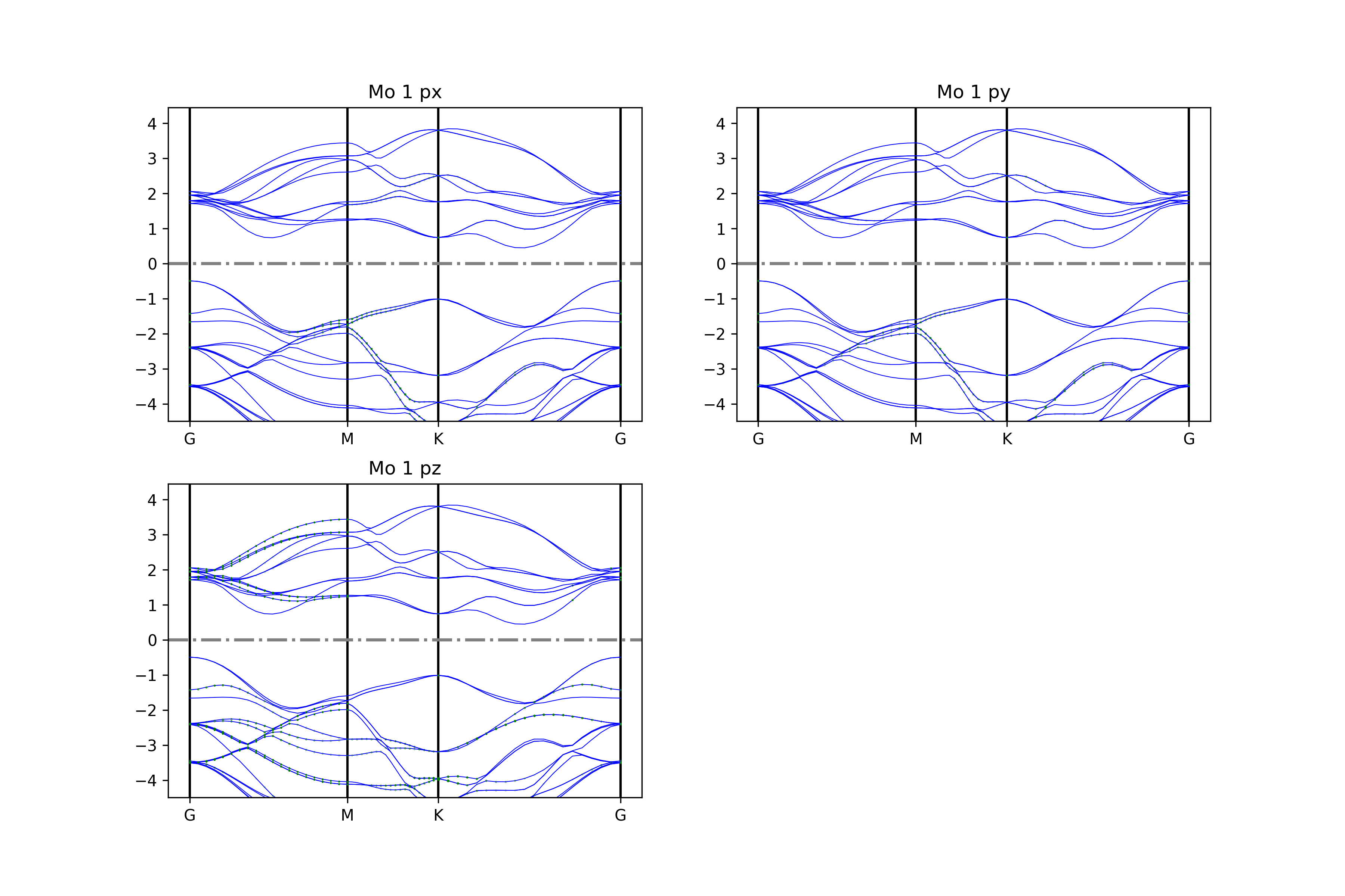
二硫化钼原子投影能带示意图

警告

如果通过SSH连接到远程服务器执行上述脚本，出现QT相关的报错信息，可能是使用的程序（比如MobaXterm等）和QT库不兼容，要么更换程序（例如VSCode或者系统自带的终端命令行），要么请在python脚本第二行开始添加以下代码：

import matplotlib
matplotlib.use('agg')

能带反折叠处理

参考 4bandunfolding.py ：

# coding:utf-8
import os

from dspawpy.plot import plot_bandunfolding

plt = plot_bandunfolding(
    datafile="dspawpy_proj/dspawpy_tests/inputs/2.22.1/band.h5",  # Read data
    ef=None,  # Fermi level, read from the file
    de=0.05,  # Band width, default 0.05
    dele=0.06,  # Band gap, default 0.06
)

plt.ylim(-15, 10)
figname = "dspawpy_proj/dspawpy_tests/outputs/us/4bandunfolding.png"  # Output band structure plot filename
os.makedirs(os.path.dirname(os.path.abspath(figname)), exist_ok=True)
plt.savefig(figname, dpi=300)
# plt.show()

执行代码可以得到类似以下能带图：

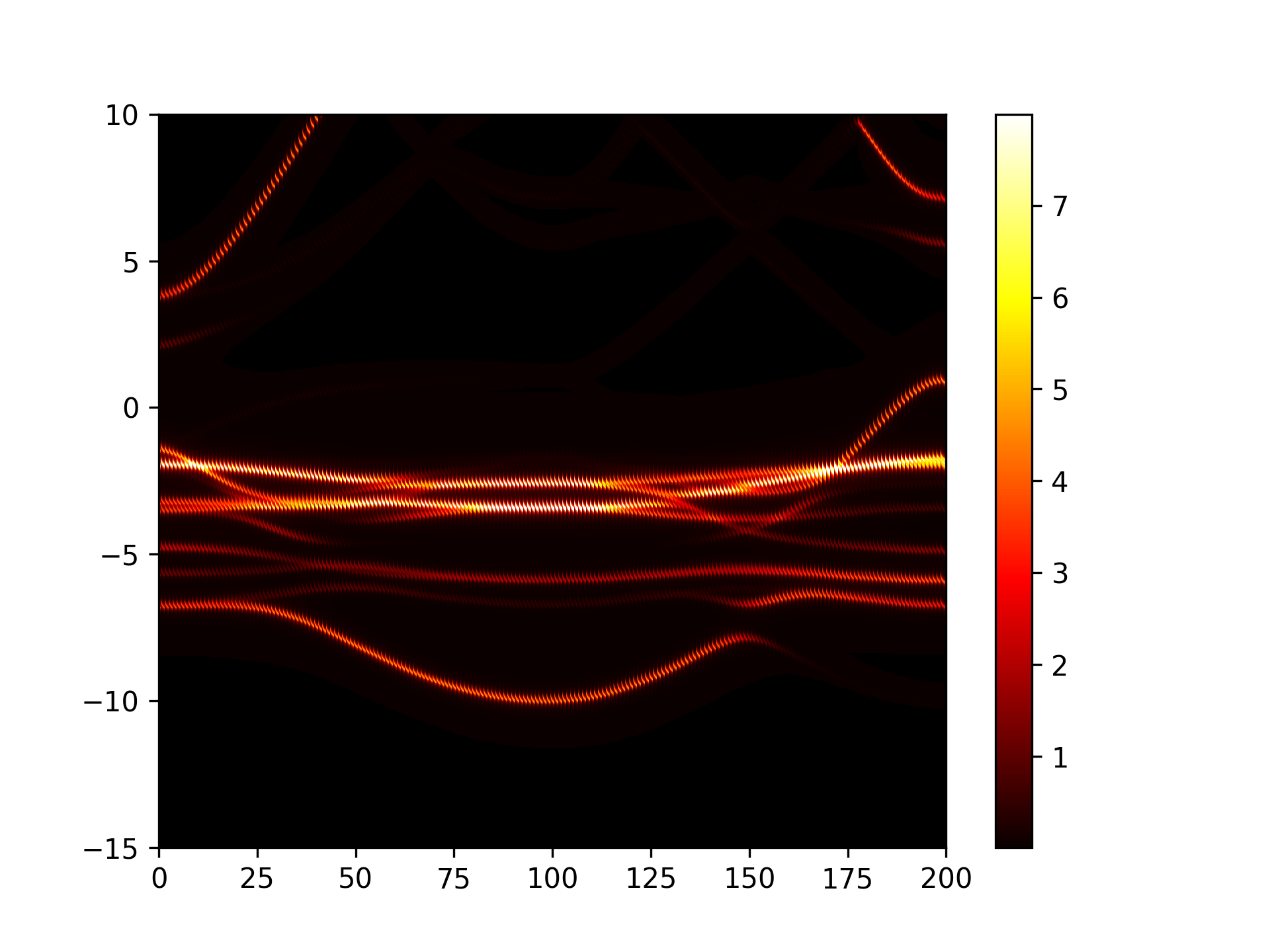
Cu3Au能带反折叠示意图

警告

此功能暂不支持将非金属材料的费米能级设为能量零点（默认价带顶为能量零点）。

警告

如果通过SSH连接到远程服务器执行上述脚本，出现QT相关的报错信息，可能是使用的程序（比如MobaXterm等）和QT库不兼容，要么更换程序（例如VSCode或者系统自带的终端命令行），要么请在python脚本第二行开始添加以下代码：

import matplotlib
matplotlib.use('agg')

band-compare能带对比图处理

将普通能带和wannier能带绘制在同一张图上

参考 4bandcompare.py ：

# coding:utf-8
import os

from pymatgen.electronic_structure.plotter import BSPlotter

from dspawpy.io.read import get_band_data

band_data = get_band_data(
    band_dir="dspawpy_proj/dspawpy_tests/inputs/2.30/wannier.h5",  # Wannier band file path
    syst_dir=None,  # system.json file path, only needed when band_dir is a json file
    efermi=None,  # Used for manually adjusting the Fermi level
    zero_to_efermi=False,  # Whether to shift zero energy to the Fermi level
)
bsp = BSPlotter(bs=band_data)
band_data = get_band_data(
    band_dir="dspawpy_proj/dspawpy_tests/inputs/2.3/band.h5",  # Read DFT band structure
    syst_dir=None,  # path to system.json file, required only when band_dir is a json file
    efermi=None,  # Used for manually correcting the Fermi level
    zero_to_efermi=False,  # Whether to shift the zero point energy to the Fermi level
)

bsp2 = BSPlotter(bs=band_data)
bsp.add_bs(bsp2._bs)
axes_or_plt = bsp.get_plot(
    zero_to_efermi=True,  # Move the zero energy level to the Fermi level
    ylim=[-10, 10],  # Energy band plot y-axis range
    smooth=False,  # Whether to smooth the band structure plot
    vbm_cbm_marker=False,  # Whether to mark the valence band maximum and conduction band minimum in the band structure plot
    smooth_tol=0,  # Threshold for smoothing
    smooth_k=3,  # Order of the smoothing process
    smooth_np=100,  # Number of points for smoothing
    bs_labels=["wannier interpolated", "DFT"],  # Band structure labels
)

import matplotlib.pyplot as plt  # noqa: E402

if isinstance(axes_or_plt, plt.Axes):
    fig = axes_or_plt.get_figure()  # version newer than v2023.8.10
else:
    fig = axes_or_plt.gcf()  # older version pymatgen

# Add a reference line for the energy zero point
for ax in fig.axes:
    ax.axhline(0, lw=2, ls="-.", color="gray")

figname = "dspawpy_proj/dspawpy_tests/outputs/us/4wanierBand.png"  # File name for the output band structure plot
os.makedirs(os.path.dirname(os.path.abspath(figname)), exist_ok=True)
fig.savefig(figname, dpi=300)

执行代码可得到类似如下能带对比曲线：

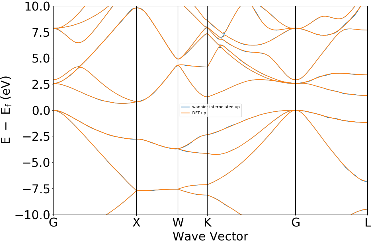
晶体硅瓦尼尔能带与DFT能带示意图

警告

如果通过SSH连接到远程服务器执行上述脚本，出现QT相关的报错信息，可能是使用的程序（比如MobaXterm等）和QT库不兼容，要么更换程序（例如VSCode或者系统自带的终端命令行），要么请在python脚本第二行开始添加以下代码：

import matplotlib
matplotlib.use('agg')

8.5 dos态密度数据处理

如有必要，参考 export_dos.py 将态密度数据提取出来并写入csv文件：

# coding:utf-8
from dspawpy.io.export import read_dos

dos_data = read_dos(
    dosfile="dspawpy_proj/dspawpy_tests/inputs/3.2.4/dos.h5",
    mode=1,  # projection mode, only valid for pdos data
    hide_index=False,  # hide index column or not
    fmt="8.3f",  # decimal format to print
)
dos_data.write_csv("dosdata.csv")

投影模式 mode 可以设置成 1~6 ，分别对应

spdf 轨道
spxpypz... 轨道
元素
原子 + spdf 轨道
原子 + spxpypz... 轨道
原子 + t2g/eg 分裂轨道

总的态密度

参考 5dosplot_total.py ：

# coding:utf-8
import os

from pymatgen.electronic_structure.plotter import DosPlotter

from dspawpy.io.read import get_dos_data
from dspawpy.plot import plot_dos

dos_data = get_dos_data(
    dos_dir="dspawpy_proj/dspawpy_tests/inputs/3.2.4/dos.h5",  # Read projected density of states data
    return_dos=False,  # If False, always return a CompleteDos object (regardless of whether projection was enabled during calculation)
)
dos_plotter = DosPlotter(
    zero_at_efermi=True,  # Whether to set the Fermi level as the zero point
    stack=False,  # True indicates drawing an area chart
    sigma=None,  # Gaussian broadening, None indicates no smoothing process
)
dos_plotter.add_dos(
    label="total dos", dos=dos_data
)  # Set the legend for the density of states plot  # Pass the density of states data

ax = plot_dos(
    dosplotter=dos_plotter,
    xlim=[-10, 5],  # Set the energy range
    ylim=[-15, 15],  # Set the density of states range
)
ax.axhline(0, lw=2, ls="-.", color="gray")

filename = "dspawpy_proj/dspawpy_tests/outputs/us/5dos_total.png"  # File name for the output density of states plot
os.makedirs(os.path.dirname(os.path.abspath(filename)), exist_ok=True)

fig = ax.get_figure()
fig.savefig(filename, dpi=300)

知识点：

使用 get_dos_data 函数可以将DS-PAW计算得到的 dos.h5 文件转化为 pymatgen 支持的格式
使用 DosPlotter模块获取到DS-PAW计算的 dos.h5 的数据
DosPlotter函数可以传递参数：stack参数表示画态密度是否加阴影， zero_at_efermi 表示是否在态密度图中进行将费米能量置零，这里设置 stack=False , zero_at_efermi=False
使用 DosPlotter 模块中 add_dos 获取态密度的数据
DosPlotter模块中 get_plot函数绘制态密度图

执行代码可以得到类似以下态密度图：

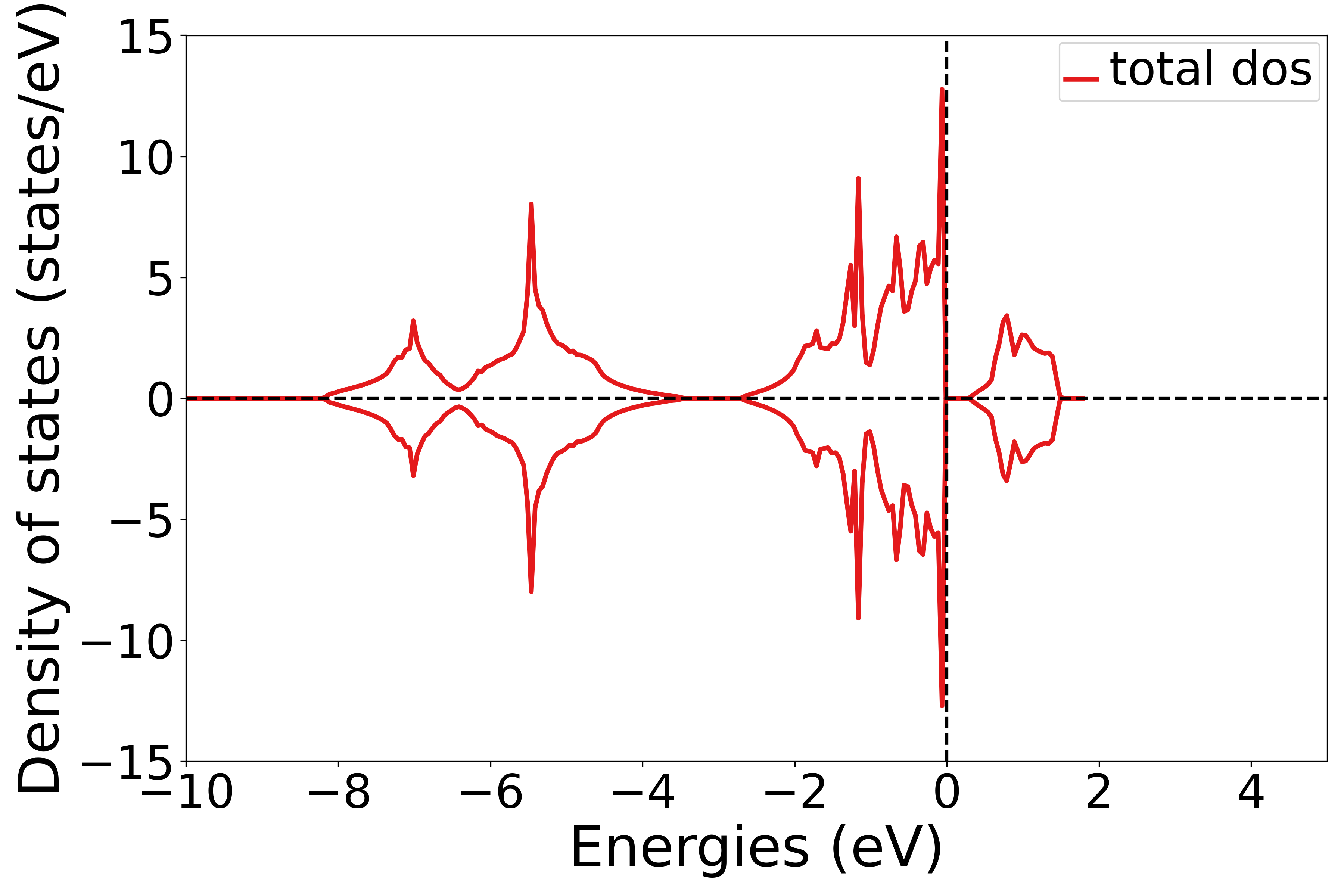
NiO态密度示意图

警告

如果通过SSH连接到远程服务器执行上述脚本，出现QT相关的报错信息，可能是使用的程序（比如MobaXterm等）和QT库不兼容，要么更换程序（例如VSCode或者系统自带的终端命令行），要么请在python脚本第二行开始添加以下代码：

import matplotlib
matplotlib.use('agg')

将态密度投影到不同的轨道上

参考 5dosplot_spd.py ：

# coding:utf-8
import os

from pymatgen.electronic_structure.plotter import DosPlotter

from dspawpy.io.read import get_dos_data
from dspawpy.plot import plot_dos

dos_data = get_dos_data(
    dos_dir="dspawpy_proj/dspawpy_tests/inputs/3.2.4/dos.h5",  # Read projected DOS data
    return_dos=False,  # If False, always return a CompleteDos object (regardless of whether projection was enabled during calculation)
)
dos_plotter = DosPlotter(
    zero_at_efermi=True,  # Whether to set the Fermi level as the zero point
    stack=False,  # True indicates drawing an area chart
    sigma=None,  # Gaussian broadening, None indicates no smoothing is applied
)
dos_plotter.add_dos_dict(
    dos_dict=dos_data.get_spd_dos(),
    key_sort_func=None,  # Orbital projection  # Specifies the sorting function
)
ax = plot_dos(
    dosplotter=dos_plotter,
    xlim=[-10, 5],  # Set the energy range
    ylim=None,  # Set the density of states range
)

ax.axhline(0, lw=2, ls="-.", color="gray")

filename = "dspawpy_proj/dspawpy_tests/outputs/us/5dos_spd.png"  # Filename of the output density of states plot
os.makedirs(os.path.dirname(os.path.abspath(filename)), exist_ok=True)

fig = ax.get_figure()
fig.savefig(filename, dpi=300)

知识点：

使用 DosPlotter模块中 add_dos_dict 函数获取投影态密度的数据，之后使用 get_spd_dos 将投影信息按照 spd 轨道投影输出

执行代码可以得到类似以下态密度图：

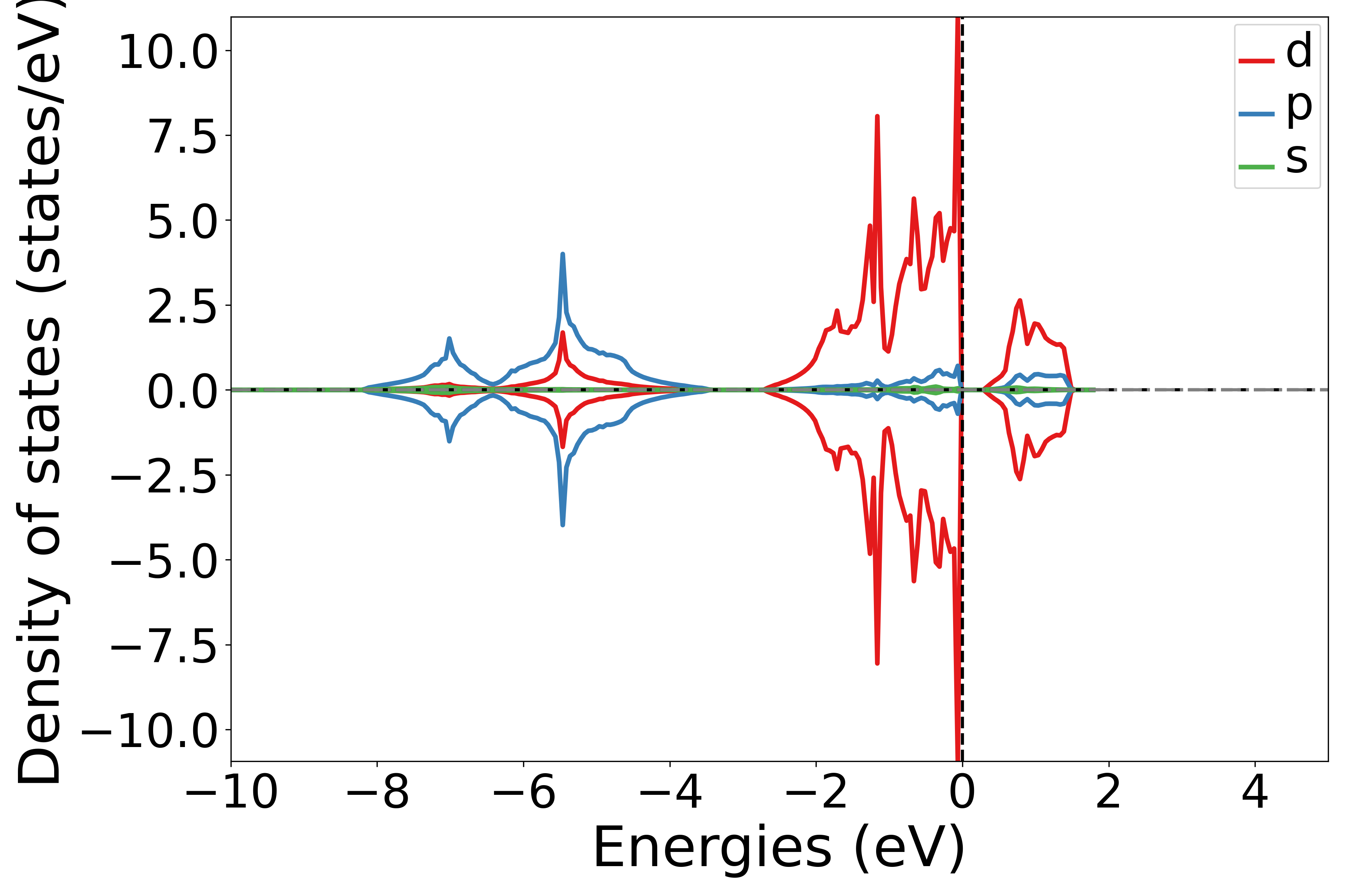
NiO轨道投影态密度示意图

警告

如果通过SSH连接到远程服务器执行上述脚本，出现QT相关的报错信息，可能是使用的程序（比如MobaXterm等）和QT库不兼容，要么更换程序（例如VSCode或者系统自带的终端命令行），要么请在python脚本第二行开始添加以下代码：

import matplotlib
matplotlib.use('agg')

将态密度投影到不同的元素上

参考 5dosplot_elt.py ：

# coding:utf-8
import os

from pymatgen.electronic_structure.plotter import DosPlotter

from dspawpy.io.read import get_dos_data
from dspawpy.plot import plot_dos

dos_data = get_dos_data(
    dos_dir="dspawpy_proj/dspawpy_tests/inputs/3.2.4/dos.h5",  # Reads projected DOS data
    return_dos=False,  # If False, always returns a CompleteDos object (regardless of whether projection was enabled during calculation)
)
dos_plotter = DosPlotter(
    zero_at_efermi=True,  # Whether to set the Fermi level as the zero point
    stack=False,  # True indicates drawing an area chart
    sigma=None,  # Gaussian broadening, None indicates no smoothing is applied
)
dos_plotter.add_dos_dict(
    dos_dict=dos_data.get_element_dos(),
    key_sort_func=None,  # Projected DOS for elements  # Specify the sorting function
)

ax = plot_dos(
    dosplotter=dos_plotter,
    xlim=[-10, 5],  # Set the energy range
    ylim=None,  # Set the density of states range
)
ax.axhline(0, lw=2, ls="-.", color="gray")

filename = "dspawpy_proj/dspawpy_tests/outputs/us/5dos_elt.png"  # Filename for the output density of states plot
os.makedirs(os.path.dirname(os.path.abspath(filename)), exist_ok=True)

fig = ax.get_figure()
fig.savefig(filename, dpi=300)

知识点：

使用 DosPlotter模块中 add_dos_dict 函数获取投影态密度的数据，之后使用 get_element_dos 将投影信息按照不同元素投影输出

执行代码可以得到类似以下态密度图：

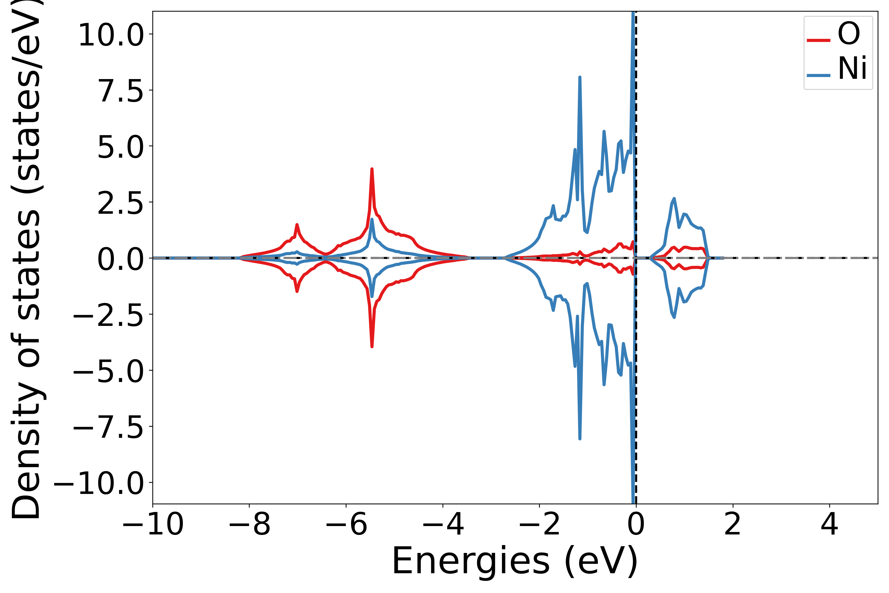
NiO元素投影态密度示意图

警告

如果通过SSH连接到远程服务器执行上述脚本，出现QT相关的报错信息，可能是使用的程序（比如MobaXterm等）和QT库不兼容，要么更换程序（例如VSCode或者系统自带的终端命令行），要么请在python脚本第二行开始添加以下代码：

import matplotlib
matplotlib.use('agg')

将态密度投影到不同原子的不同轨道上

参考 5dosplot_atom_orbit.py ：

# coding:utf-8
import os

from pymatgen.electronic_structure.core import Orbital
from pymatgen.electronic_structure.plotter import DosPlotter

from dspawpy.io.read import get_dos_data
from dspawpy.plot import plot_dos

dos_data = get_dos_data(
    dos_dir="dspawpy_proj/dspawpy_tests/inputs/3.2.4/dos.h5",  # Reads projected density of states data
    return_dos=False,  # If False, always return a CompleteDos object (regardless of whether projection was enabled during calculation)
)
dos_plotter = DosPlotter(
    zero_at_efermi=True,  # Whether to set the Fermi level as the zero point
    stack=False,  # True indicates drawing an area plot
    sigma=None,  # Gaussian broadening, None indicates no smoothing treatment
)

# ! Specify atomic number and orbital
dict_index_orbit = {0: ["dxy"], 2: ["s"]}

print("Plotting...")
for index in dict_index_orbit:
    _os = dict_index_orbit[index]
    _e = str(dos_data.structure.sites[index].species)
    for _orb in _os:
        dos_plotter.add_dos(
            f"{_e}(atom-{index}) {_orb}",  # label
            dos_data.get_site_orbital_dos(
                dos_data.structure[index],
                getattr(Orbital, _orb),
            ),
        )

ax = plot_dos(
    dosplotter=dos_plotter,
    xlim=[-10, 5],  # Set the energy range
    ylim=None,  # Set the density of states range
)
ax.axhline(0, lw=2, ls="-.", color="gray")

figname = "dspawpy_proj/dspawpy_tests/outputs/us/5dos_atom_orbit.png"  # Output density of states figure filename
os.makedirs(os.path.dirname(os.path.abspath(figname)), exist_ok=True)

fig = ax.get_figure()
fig.savefig(figname, dpi=300)

知识点：

使用 get_site_orbital_dos函数提取dos数据中特定原子特定轨道的贡献，dos_data.structure[0],Orbital(4) 表示获取第1个原子的dxy轨道的态密度，get_site_orbital_dos函数中序号从0开始
运行此脚本，根据提示选择元素和轨道，可以得到相应的态密度图

执行代码可以得到类似以下态密度图：

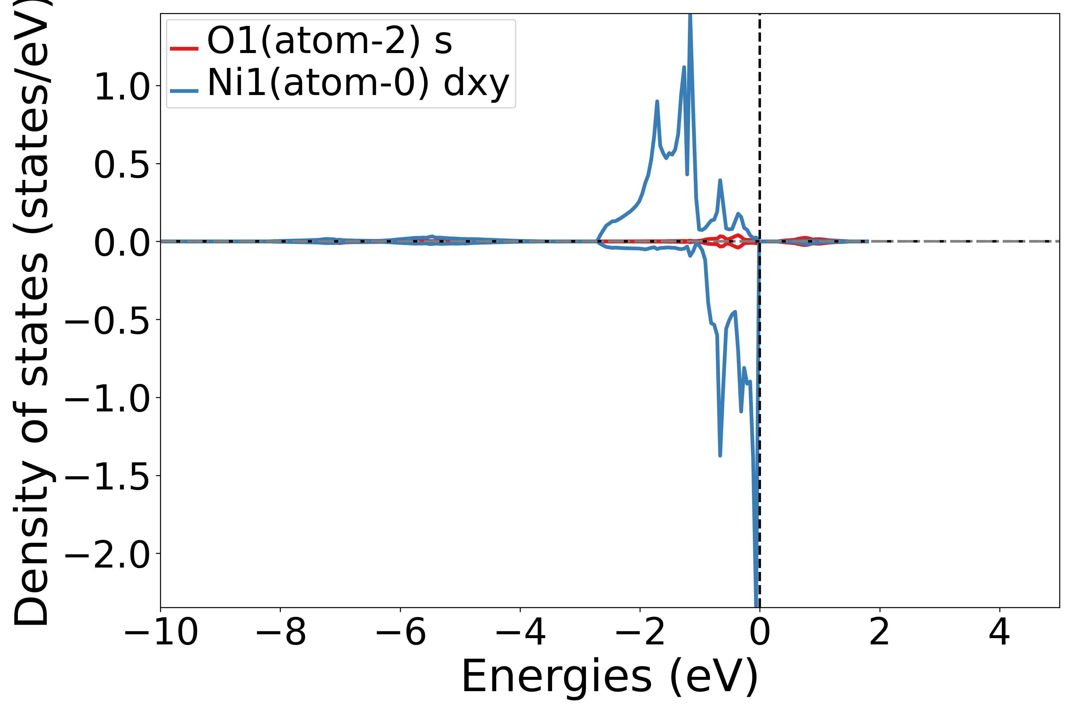
NiO原子轨道态密度示意图

警告

如果通过SSH连接到远程服务器执行上述脚本，出现QT相关的报错信息，可能是使用的程序（比如MobaXterm等）和QT库不兼容，要么更换程序（例如VSCode或者系统自带的终端命令行），要么请在python脚本第二行开始添加以下代码：

import matplotlib
matplotlib.use('agg')

将态密度投影到不同原子的分裂d轨道(t2g, eg)上

参考 5dosplot_t2g_eg.py ：

# coding:utf-8
import os

from pymatgen.electronic_structure.plotter import DosPlotter

from dspawpy.io.read import get_dos_data
from dspawpy.plot import plot_dos

dos_data = get_dos_data(
    dos_dir="dspawpy_proj/dspawpy_tests/inputs/3.2.4/dos.h5",  # Read projected density of states data
    return_dos=False,  # If False, always returns a CompleteDos object (regardless of whether projection was enabled during calculation)
)
dos_plotter = DosPlotter(
    zero_at_efermi=True,  # Whether to set the Fermi level as the zero point
    stack=False,  # True indicates drawing an area chart
    sigma=None,  # Gaussian broadening, None indicates no smoothing is applied
)
# print(dos_data.structure)

# Specify the atomic number, starting from 0
ais = [1]

print("Plotting...")
atom_indices = [int(ai) for ai in ais]
for atom_index in atom_indices:
    dos_plotter.add_dos_dict(
        dos_data.get_site_t2g_eg_resolved_dos(dos_data.structure[atom_index]),
    )

ax = plot_dos(
    dosplotter=dos_plotter,
    xlim=[-10, 5],  # Set the energy range
    ylim=None,  # Set the density of states range
)
ax.axhline(0, lw=2, ls="-.", color="gray")

filename = "dspawpy_proj/dspawpy_tests/outputs/us/5dos_t2g_eg.png"  # Output density of states plot filename
os.makedirs(os.path.dirname(os.path.abspath(filename)), exist_ok=True)

fig = ax.get_figure()
fig.savefig(filename, dpi=300)

知识点：

使用 get_site_t2g_eg_resolved_dos函数提取dos数据中特定原子的 t2g和 eg轨道的贡献，这是获取第2个原子的t2g和eg轨道的贡献
运行此脚本，根据提示选择原子序号，可以得到相应的态密度图

执行代码可以得到类似以下态密度图：

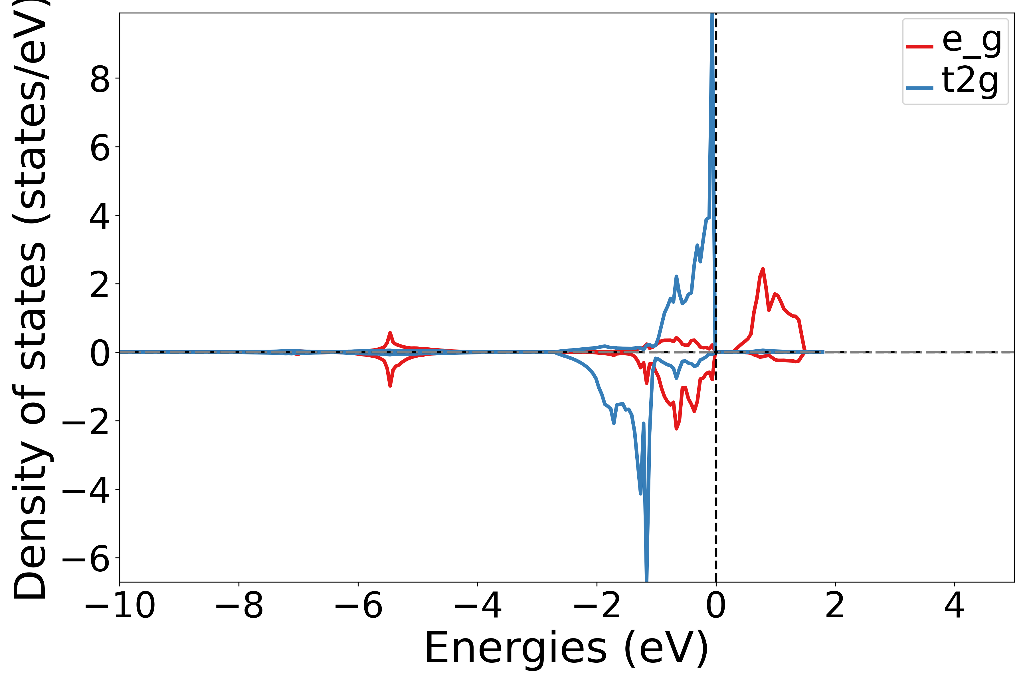
NiO分裂d轨道原子投影态密度示意图

知识点：

如果元素不含d轨道，会画成空白图片

警告

如果通过SSH连接到远程服务器执行上述脚本，出现QT相关的报错信息，可能是使用的程序（比如MobaXterm等）和QT库不兼容，要么更换程序（例如VSCode或者系统自带的终端命令行），要么请在python脚本第二行开始添加以下代码：

import matplotlib
matplotlib.use('agg')

d-带中心分析

以 Pb-slab 体系为例，对 Pt 原子进行 d-band 中心分析：

参考 5center_dband.py ：

# coding:utf-8
from dspawpy.io.read import get_dos_data
from dspawpy.io.utils import d_band

dos_data = get_dos_data(
    dos_dir="dspawpy_proj/dspawpy_tests/inputs/supplement/dos.h5",  # Read projected density of states data
    return_dos=False,  # If False, always returns a CompleteDos object (regardless of whether projection was enabled during calculation)
)
for spin in dos_data.densities:
    print("spin=", spin)
    c = d_band(spin, dos_data)
    print(c)

执行代码可以得到类似以下结果：

spin=1
-1.785319344084034

备注

目前仅支持全部原子平均的 d 轨道中心，不支持元素、原子投影或其他轨道，也不支持选择自旋方向或能量范围。

get_dos_data 函数负责处理态密度数据：

8.6 bandDos能带和态密度共同显示

以应用教程中Si体系为例：

将能带和态密度显示在一张图上

参考 6bandDosplot.py ：

# coding:utf-8
import os

import numpy as np
from matplotlib.axes import Axes
from pymatgen.electronic_structure.plotter import BSDOSPlotter

from dspawpy.io.read import get_band_data, get_dos_data

bandfile = "dspawpy_proj/dspawpy_tests/inputs/2.3/band.h5"  # Normal band data
band_data = get_band_data(
    band_dir=bandfile,
    syst_dir=None,  # path to system.json file, required only when band_dir is a json file
    efermi=None,  # Used for manually correcting the Fermi level
)
band_efermi = band_data.efermi
dosfile = "dspawpy_proj/dspawpy_tests/inputs/2.5/dos.h5"  # Density of states data
dos_data = get_dos_data(
    dos_dir=dosfile,
    return_dos=False,  # If False, always return a CompleteDos object (regardless of whether projection was enabled during calculation)
)
dos_efermi = dos_data.efermi
bdp = BSDOSPlotter(
    bs_projection=None,  # Band structure projection method, None means no projection
    dos_projection=None,  # Projection method for density of states, None means no projection
    vb_energy_range=4,  # Valence band energy range
    cb_energy_range=4,  # Conduction band energy range
    fixed_cb_energy=False,  # Whether to fix the conduction band energy range
    egrid_interval=1,  # Energy grid interval
    font="DejaVu Sans",  # Default is Times New Roman, change to DejaVu Sans to avoid warnings due to missing font on Linux
    axis_fontsize=20,  # Axis font size
    tick_fontsize=15,  # Tick label font size
    legend_fontsize=14,  # Legend font size
    bs_legend="best",  # Band structure legend position
    dos_legend="best",  # Density of States legend position
    rgb_legend=True,  # Use colored legend
    fig_size=(11, 8.5),  # Figure size
)
if band_efermi != dos_efermi:
    print(f"{band_efermi=:.4f} eV")
    print(f"{dos_efermi=:.4f} eV")
    d_efermi = band_efermi - dos_efermi

    print(
        "! Band and DOS Fermi levels are inconsistent, using DOS Fermi level as reference"
    )
    band_data.bands = {spin: v + d_efermi for spin, v in band_data.bands.items()}

    # ! Band and DOS Fermi levels are inconsistent, using Band level as the reference
    # dos_data.energies -= d_efermi

axes_or_plt = bdp.get_plot(
    bs=band_data, dos=dos_data
)  # Pass band data  # Pass density of states data

if isinstance(axes_or_plt, Axes):
    fig = axes_or_plt.get_figure()  # version newer than v2023.8.10
elif np.iterable(axes_or_plt):
    fig = np.asarray(axes_or_plt).flatten()[0].get_figure()
else:
    fig = axes_or_plt.gcf()  # older version pymatgen

filename = "dspawpy_proj/dspawpy_tests/outputs/us/6bandDos.png"  # Filename for the band structure - density of states plot output
os.makedirs(os.path.dirname(os.path.abspath(filename)), exist_ok=True)
fig.savefig(filename, dpi=300)
print("==> Saved", filename)

执行代码可以得到类似以下能带态密度图：

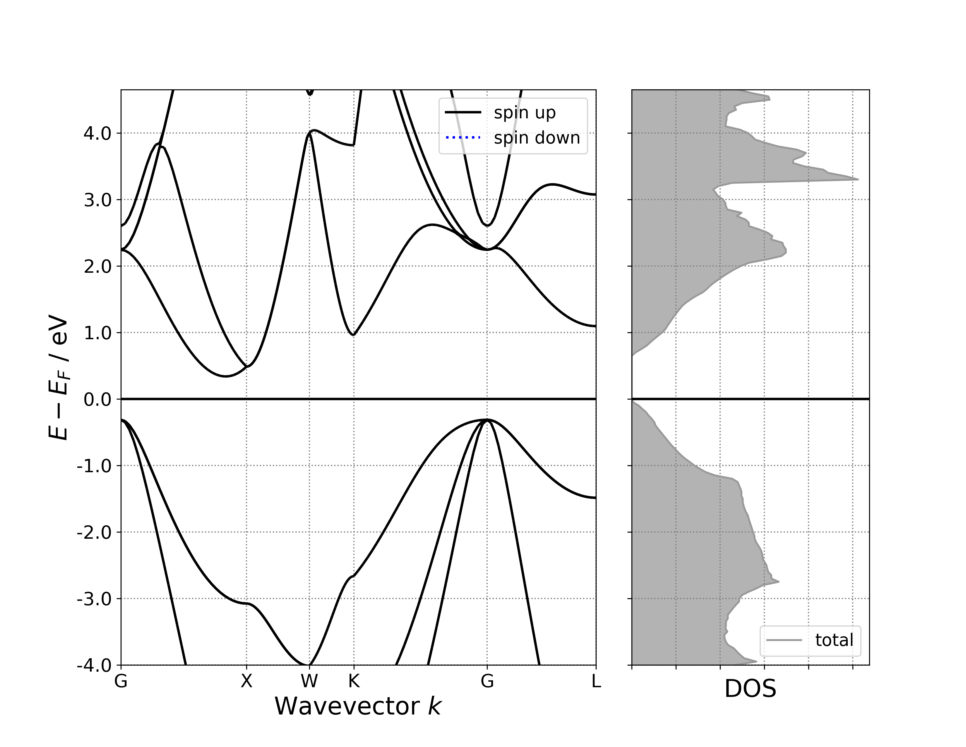
单晶硅能带-态密度示意图

警告

如果通过SSH连接到远程服务器执行上述脚本，出现QT相关的报错信息，可能是使用的程序（比如MobaXterm等）和QT库不兼容，要么更换程序（例如VSCode或者系统自带的终端命令行），要么请在python脚本第二行开始添加以下代码：

import matplotlib
matplotlib.use('agg')

将能带和投影态密度显示在一张图上

参考 6bandPdosplot.py ：

# coding:utf-8
import os

import numpy as np
from matplotlib.axes import Axes
from pymatgen.electronic_structure.plotter import BSDOSPlotter

from dspawpy.io.read import get_band_data, get_dos_data

bandfile = "dspawpy_proj/dspawpy_tests/inputs/2.4/band.h5"  # Normal band data
band_data = get_band_data(
    band_dir=bandfile,
    syst_dir=None,  # path to system.json file, required only when band_dir is a json file
    efermi=None,  # Used for manually correcting the Fermi level
)
band_efermi = band_data.efermi
dosfile = (
    "dspawpy_proj/dspawpy_tests/inputs/2.6/dos.h5"  # DOS data for projected states
)
dos_data = get_dos_data(
    dos_dir=dosfile,
    return_dos=False,  # If False, always return a CompleteDos object (regardless of whether projection was enabled during calculation)
)
dos_efermi = dos_data.efermi
bdp = BSDOSPlotter(
    bs_projection="elements",  # Projection method for band structure, None means no projection
    dos_projection="elements",  # Project DOS onto elements
    vb_energy_range=4,  # Valence band energy range
    cb_energy_range=4,  # Conduction band energy range
    fixed_cb_energy=False,  # Whether to fix the conduction band energy range
    egrid_interval=1,  # Energy grid interval
    font="DejaVu Sans",  # Default is Times New Roman, can be changed to DejaVu Sans to avoid warnings due to font not being installed on Linux
    axis_fontsize=20,  # Axis font size
    tick_fontsize=15,  # Tick label font size
    legend_fontsize=14,  # Legend font size
    bs_legend="best",  # Band structure legend position
    dos_legend="best",  # Position of the projected density of states legend
    rgb_legend=True,  # Use colored legend
    fig_size=(11, 8.5),  # Figure size
)
if band_efermi != dos_efermi:
    print(f"{band_efermi=:.4f} eV")
    print(f"{dos_efermi=:.4f} eV")
    d_efermi = band_efermi - dos_efermi

    print(
        "! Band and DOS Fermi levels are inconsistent, using DOS Fermi level as reference"
    )
    band_data.bands = {spin: v + d_efermi for spin, v in band_data.bands.items()}

    # ! Band and DOS Fermi levels are inconsistent, using Band level as reference
    # dos_data.energies -= d_efermi

axes_or_plt = bdp.get_plot(
    bs=band_data,
    dos=dos_data,
)  # Pass band structure data  # Pass projected density of states data

if isinstance(axes_or_plt, Axes):
    fig = axes_or_plt.get_figure()  # version newer than v2023.8.10
elif np.iterable(axes_or_plt):
    fig = np.asarray(axes_or_plt).flatten()[0].get_figure()
else:
    fig = axes_or_plt.gcf()  # older version pymatgen

filename = "dspawpy_proj/dspawpy_tests/outputs/us/6bandPdos.png"  # filename for the band structure-projected density of states plot
os.makedirs(os.path.dirname(os.path.abspath(filename)), exist_ok=True)
fig.savefig(filename, dpi=300)
print("==> Saved", filename)

执行代码可以得到类似以下能带态密度图：

单晶硅能带-投影态密度示意图

警告

给定投影能带数据，默认将沿着元素投影；给定普通能带数据（或体系所含元素种类超过4种），则不投影，并输出警告
给定投影态密度数据，默认也将沿着元素投影，可以换成沿着轨道投影，或者不投影；给定普通态密度数据且未关闭态密度投影选项 BSDOSPlotter(dos_projection=None)，pymatgen绘图程序将报错，这就是上面特意准备了一个 6bandDosplot.py 文件的原因。

警告

如果通过SSH连接到远程服务器执行上述脚本，出现QT相关的报错信息，可能是使用的程序（比如MobaXterm等）和QT库不兼容，要么更换程序（例如VSCode或者系统自带的终端命令行），要么请在python脚本第二行开始添加以下代码：

import matplotlib
matplotlib.use('agg')

8.7 optical光学性质数据处理

以快速入门Si体系光学性质计算得到的 scf.h5 为例（注：输出文件名与task一致，task = scf，io.optical = true可计算光学性质）：

反射率数据处理，参考 7optical.py ：

# coding:utf-8
from dspawpy.plot import plot_optical

plot_optical(
    datafile="dspawpy_proj/dspawpy_tests/inputs/2.12/scf.h5",
    keys=["ExtinctionCoefficient", "Reflectance"],
    axes=["X"],  # ["X", "Y", "Z", "XY", "YZ", "ZX"]
    prefix="dspawpy_proj/dspawpy_tests/outputs/optical",  # Where to save, if empty, it means the current folder
    save=True,  # Whether to save the image with the tool's name, if False, please refer to the script below to save manually
)

# The above function will plot and save the images of ExtinctionCoefficient and Reflectance separately
# To plot multiple properties on the same figure, uncomment the following code and set the save parameter above to False

# import os
# import matplotlib.pyplot as plt
#
# plt.tick_params(labelsize=16)
# plt.tight_layout()
# filename = "outputs/us/7optical.png"  # Filename for the output optical properties plot
# os.makedirs(os.path.dirname(os.path.abspath(filename)), exist_ok=True)
# plt.savefig(filename, dpi=300)

知识点：

Reflectance为光学性质中的一种，用户可以根据自己的需求将该关键词修改为“AbsorptionCoefficient”或”ExtinctionCoefficient”或”RefractiveIndex”，分别对应吸收系数、消光系数和折射率

执行代码可以得到类似以下反射率随能量变化的曲线：

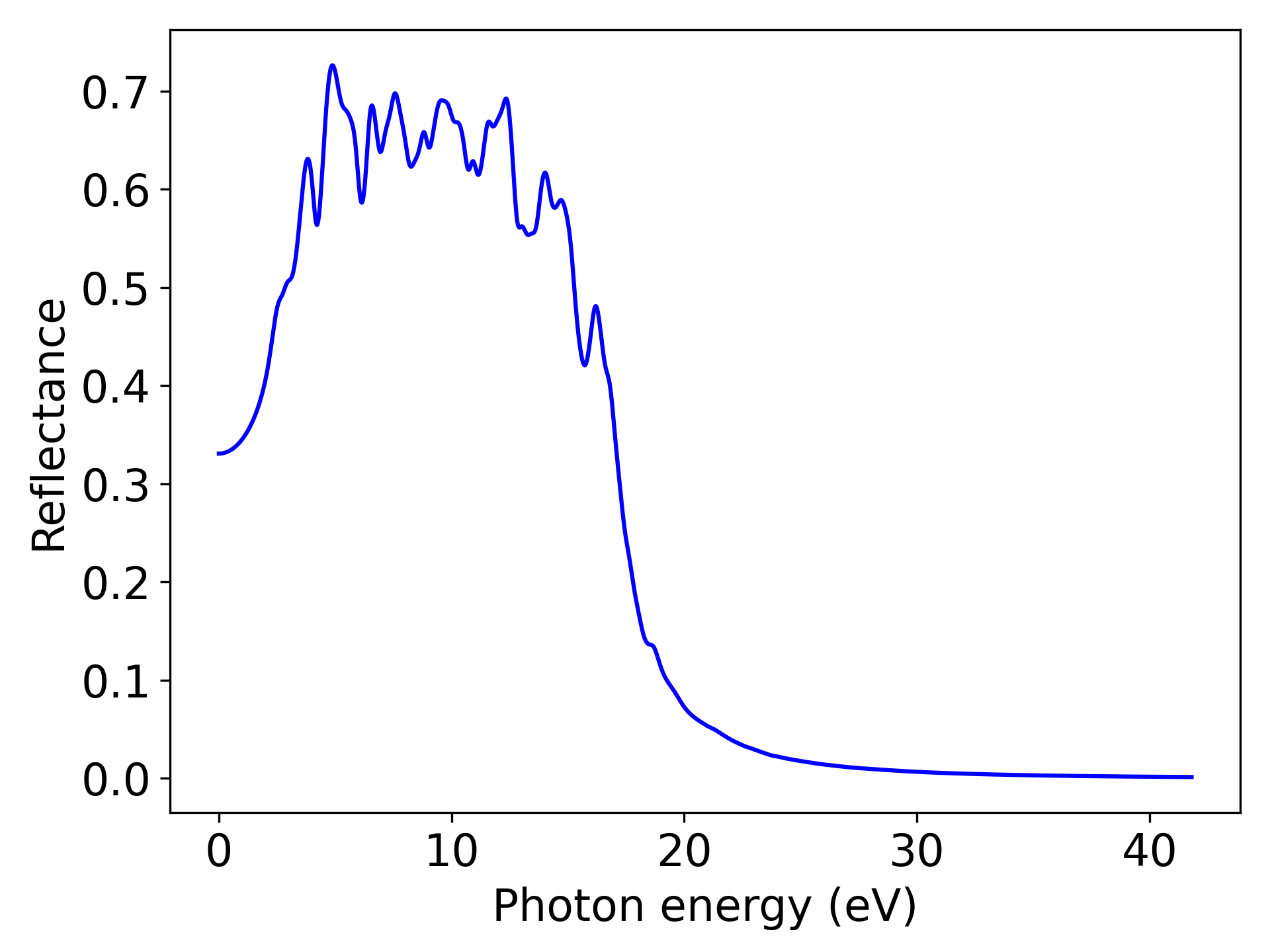
单晶硅Reflectance随光子能量变化趋势示意图

警告

如果通过SSH连接到远程服务器执行上述脚本，出现QT相关的报错信息，可能是使用的程序（比如MobaXterm等）和QT库不兼容，要么更换程序（例如VSCode或者系统自带的终端命令行），要么请在python脚本第二行开始添加以下代码：

import matplotlib
matplotlib.use('agg')

8.8 neb过渡态计算数据处理

以快速入门 H 在 Pt(100) 表面扩散为例进行介绍：

输入文件之生成中间构型

参考 8neb_interpolate_structures.py ：

# coding:utf-8
from dspawpy.diffusion.neb import NEB, write_neb_structures
from dspawpy.diffusion.nebtools import write_json_chain
from dspawpy.io.structure import read

# Read initial configuration
init_struct = read("dspawpy_proj/dspawpy_tests/inputs/2.15/00/structure00.as")[0]
# Read final state configuration
final_struct = read("dspawpy_proj/dspawpy_tests/inputs/2.15/04/structure04.as")[0]

neb = NEB(
    initial_structure=init_struct,  # Initial structure
    final_structure=final_struct,  # Final state configuration
    nimages=8,  # Total of 8 configurations, including initial and final states
)
structures = neb.linear_interpolate()  # Linear interpolation
# structures = neb.idpp_interpolate()   # IDPP interpolation

# Save as structure file to dest path
write_neb_structures(
    structures=structures,  # Insert interpolated structure chains
    coords_are_cartesian=True,  # Whether to save in Cartesian coordinates
    fmt="as",  # Save format, supported formats: 'json', 'as', 'hzw', 'pdb', 'xyz', 'dump'
    path="dspawpy_proj/dspawpy_tests/outputs/us/8neb_interpolate_structures",  # Save path
    prefix="structure",  # File name prefix
)

# Preview initial structure chain
write_json_chain(
    preview=True,  # whether to enable preview mode
    directory="dspawpy_proj/dspawpy_tests/outputs/us/8neb_interpolate_structures",  # Directory for NEB calculations
    step=-1,  # Default to saving the structure chain of the last ion step (latest)
    dst="dspawpy_proj/dspawpy_tests/outputs/us/8neb",  # Save path
)
# write_xyz_chain(preview=True, # Whether to run in preview mode
#                  directory="dspawpy_proj/dspawpy_tests/outputs/us/8neb_interpolate_structures", # NEB calculation directory
#                  step=-1, # Default to saving the structure chain of the last ionic step (latest)
#                  dst='dspawpy_proj/dspawpy_tests/outputs/us/8neb' # save path
# )

知识点：

用户可以根据需要自行修改插点个数，设置为8得到包含8个结构文件的文件夹，其中中间构型为6个
neb.linear_interpolate为线性插值方法，pbc参数为 True 时将锁定寻找最短扩散路径，默认为 False 以增加用户控制的灵活性，这是因为
举个例子，初态某原子的分数坐标是 0.2，终态变成 0.8。pbc = True 将强制设置扩散路径为 0.2 -> -0.2。pbc = False 则用户可以令程序按照 0.2 -> 0.8 的扩散路径进行插值；如果要用最短路径，手动将 0.8 改为 -0.2 即可，从而确保程序按照使用者的意图完成插值初猜。

绘制能垒图

neb.iniFin = true/false

当设置 neb.iniFin = true/false 时，都可使用读取neb计算的路径进行势垒分析（确保初末态计算文件在neb计算路径下）：

参考 8neb_barrier_CubicSpline.py ：

# coding:utf-8
from dspawpy.diffusion.nebtools import plot_barrier

directory_of_neb_task = (
    "dspawpy_proj/dspawpy_tests/inputs/2.15"  # <-- Please modify to the actual NEB path
)

# Plotting the energy barrier using CubicSpline interpolation
plot_barrier(
    directory=directory_of_neb_task,  # path of the neb task
    method="CubicSpline",  # Cubic spline interpolation
    figname="dspawpy_proj/dspawpy_tests/outputs/us/8neb_barrier_CubicSpline.png",  # Output filename for the energy barrier plot
    show=False,  # Whether to display the energy barrier plot
)

备注

运行上述脚本后，可得到类似以下三次样条插值的势垒曲线：

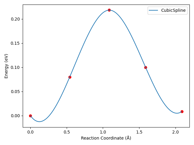
对于这个算例，三次样条插值后，曲线会出现不合理的“下坠”区域，这是三次样条插值算法的特性所决定的。

dspawpy 内部调用 scipy 的插值算法，上面这个脚本我们以三次样条插值算法为例，它在 scipy 文档中的定义为：

class scipy.interpolate.CubicSpline(x, y, axis=0, bc_type='not-a-knot', extrapolate=None)

关键词参数包括 axis, bc_type, extrapolate，具体含义见 scipy.interpolate.CubicSpline 。我们可以往 plot_barrier 函数中指定相应的关键词参数（axis, bc_type, extrapolate），将其传递给 scipy.interpolate.CubicSpline 这个类处理。

下面我们采用 8neb_barrier.py 脚本，对比三种算法插值绘制出的曲线：

# coding:utf-8
import os

import matplotlib.pyplot as plt

from dspawpy.diffusion.nebtools import plot_barrier

# Compare the differences in energy barrier curves drawn by different interpolation methods, where show should be set to False
# 1. interp1d
plot_barrier(
    directory="dspawpy_proj/dspawpy_tests/inputs/2.15",  # path for NEB calculation
    ri=None,  # Reaction coordinate between the initial structure and the second structure, required when the NEB task only calculated intermediate structures
    rf=None,  # Reaction coordinate between the last configuration and the second-to-last configuration, when the NEB task only calculated intermediate configurations
    ei=None,  # Energy of the initial configuration, required when the NEB task only calculated intermediate configurations
    ef=None,  # Energy of the final configuration, required when the NEB task only calculated intermediate configurations
    method="interp1d",  # Interpolation method
    figname=None,  # Name of the output energy barrier plot file
    show=False,  # Whether to display the energy barrier plot
    kind="quadratic",  # Parameter of the interpolation method
)
# 2. CubicSpline
plot_barrier(
    directory="dspawpy_proj/dspawpy_tests/inputs/2.15",
    method="CubicSpline",
    figname=None,
    show=False,
)
# 3. pchip
plot_barrier(
    directory="dspawpy_proj/dspawpy_tests/inputs/2.15",
    method="pchip",
    figname=None,
    show=False,
)

filename = "dspawpy_proj/dspawpy_tests/outputs/us/8neb_barrier_comparison.png"  # Filename for the energy barrier plot output
os.makedirs(os.path.dirname(os.path.abspath(filename)), exist_ok=True)
plt.savefig(filename, dpi=300)
# plt.show()

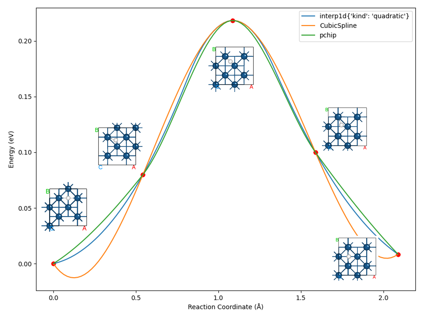
知识点：

选择合适的插值算法对于优化最终曲线的呈现效果至关重要
多数情况下，选择 pchip 这种单调三次样条插值算法即可达到较好效果，这也是默认调用的插值算法

neb.iniFin = true

当设置 neb.iniFin = true 时，读取neb计算所得的 neb.h5/neb.json 文件可快速进行势垒分析：

参考 8neb_barrier_CubicSpline.py ：

# coding:utf-8
from dspawpy.diffusion.nebtools import plot_barrier

# Plot energy barrier using CubicSpline interpolation
plot_barrier(
    datafile="dspawpy_proj/dspawpy_tests/inputs/2.15/neb.h5",  # Path to neb.h5
    method="CubicSpline",  # Cubic spline interpolation
    figname="dspawpy_proj/dspawpy_tests/outputs/us/8neb_barrier_.png",  # Output file name for the energy barrier plot
    show=False,  # Whether to display the energy barrier plot
)

处理得到的势垒图与之前读取路径效果一致。

备注

neb.h5 和 neb.json文件所存能量为TotalEnergy，如需得精确的势垒值，建议采用读取neb计算路径的方法进行处理（取TotalEnergy0）

警告

如果通过SSH连接到远程服务器执行上述脚本，出现QT相关的报错信息，可能是使用的程序（比如MobaXterm等）和QT库不兼容，要么更换程序（例如VSCode或者系统自带的终端命令行），要么请在python脚本第二行开始添加以下代码：

import matplotlib
matplotlib.use('agg')

过渡态计算数据处理

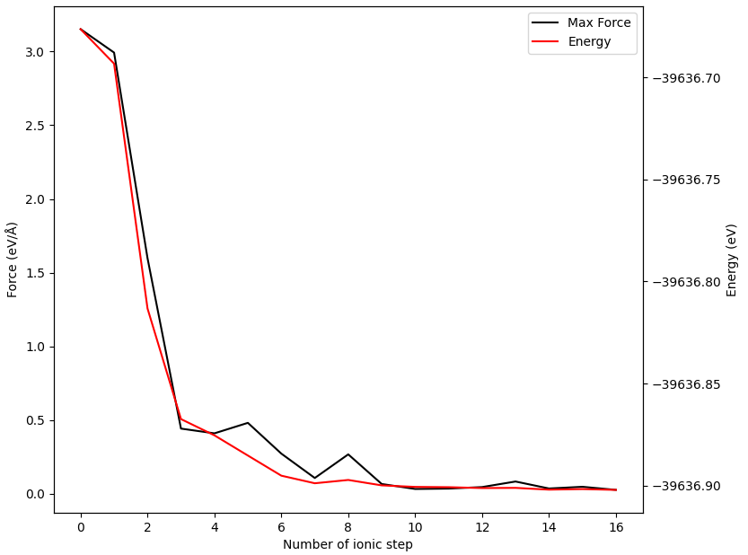
NEB计算完成后，一般要画出能垒图观察，并检查各插值构型最终的受力大小，从而确保受力小于指定的阈值。如果结果异常，还需要检查各插值构型在结构优化过程中的受力与能量变化趋势，判断是否真正“收敛”。上述这些操作至少需要三次循环，为简化操作，我们提供了一个一步到位的总结函数 summary ：

参考 8neb_check_results.py ：

# coding:utf-8
from dspawpy.diffusion.nebtools import summary

# Import the neb calculation directory, a complete folder after neb calculation needs to be provided
summary(
    directory="dspawpy_proj/dspawpy_tests/inputs/2.15",
    show_converge=False,  # Whether to display the convergence plots of energy and force
    outdir="dspawpy_proj/dspawpy_tests/outputs/us/8neb",  # Path to save convergence plots of energy and forces
    figname="dspawpy_proj/dspawpy_tests/outputs/us/8neb/neb_barrier_summary.png",  # Path to save the energy barrier plot
)
# Additional keyword arguments can be set for plotting the barrier diagram, such as:
# summary(directory='dspawpy_proj/dspawpy_tests/inputs/2.15', method='CubicSpline') # Change to CubicSpline for spline interpolation

知识点：

此脚本将以表格形式打印各构型的能量和受力、绘制能垒图，并绘制中间构型的能量与受力收敛过程图
若 neb.iniFin = false ，用户必须将自洽计算的结果文件 scf.h5 或 system.json 文件复制到对应的初末态子文件夹中，否则程序无法读取初末态能量和受力信息，将报错退出
默认情况下，能垒图存储在neb计算目录外层，各中间构型的能量与受力收敛图存储在各子文件夹

执行代码可以得到类似如下NEB计算各构型的能量和受力表格：

Image	Force (eV/Å)	Reaction coordinate (Å)	Energy (eV)	Delta energy (eV)
00	0.1803	0.0000	-39637.0984	0.0000
01	0.0263	0.5428	-39637.0186	0.0798
02	0.0248	1.0868	-39636.8801	0.2183
03	0.2344	1.5884	-39636.9984	0.1000
04	0.0141	2.0892	-39637.0900	0.0084

除了可以获得能垒图外，还可以得到各中间构型的能量和受力收敛曲线（以02构型为例）

警告

如果通过SSH连接到远程服务器执行上述脚本，出现QT相关的报错信息，可能是使用的程序（比如MobaXterm等）和QT库不兼容，要么更换程序（例如VSCode或者系统自带的终端命令行），要么请在python脚本第二行开始添加以下代码：

import matplotlib
matplotlib.use('agg')

观察NEB链

此处所说NEB链指的是各插值构型（structure00.as, structure01.as, ...）之间的几何关系，而不是单个构型在优化过程中的变化。

NEB任务计算量较大，观察NEB链有助于判断NEB计算的收敛速度。另外，通过插值算法生成中间结构后，经常需要预览NEB链。这些需求可以通过 8neb_visualize.py 脚本实现：

# coding:utf-8
from dspawpy.diffusion.nebtools import write_json_chain, write_xyz_chain

# Convert the configuration chain under the NEB calculation path to a JSON format file
write_json_chain(
    preview=False,  # If the NEB calculation is already completed, preview mode is not required
    directory="dspawpy_proj/dspawpy_tests/inputs/2.15",  # NEB calculation directory
    step=-1,  # Default to saving the configuration chain of the last ion step (latest)
    dst="dspawpy_proj/dspawpy_tests/outputs/us/8neb",  # Save path
    ignorels=False,  # Set to True to ignore latestStructureXX.as files
)

# Convert the configuration chain in the NEB calculation path to xyz format files
write_xyz_chain(
    preview=False,  # If the NEB calculation is already completed, preview mode is not required
    directory="dspawpy_proj/dspawpy_tests/inputs/2.15",  # NEB calculation directory
    step=-1,  # Default to saving the configuration chain of the last ionic step (latest)
    dst="dspawpy_proj/dspawpy_tests/outputs/us/8neb",  # Save path
    ignorels=False,  # Set to True to ignore latestStructureXX.as files
)

知识点：

此脚本生成neb_movie*.json文件后，通过 Device Studio --> Simulator --> DS-PAW --> Analysis Plot 打开 json 文件即可观察
directory指定为NEB计算主路径，需提供neb计算完成后的完整文件夹
该脚本支持处理正在进行中的（即未完成的）neb计算文件，方便用户监测实时轨迹
xyz文件可通过 OVITO 软件打开查看：通过 Device Studio --> Simulator --> OVITO 打开可视化界面，将xyz文件拖入即可
结构信息读取优先级：latestStructureXX.as > h5 > json；设置ignorels为True后，先尝试读取 h5 中的数据，失败则读取 json 中的数据

计算构型间距

参考这个脚本 8calc_dist.py ：

# coding:utf-8
from dspawpy.diffusion.nebtools import get_distance
from dspawpy.io.structure import read

# Please modify the paths of structure01.as and structure02.as structure files according to the actual situation
# First read the fractional coordinates, element list, and cell information of the two configurations
s1 = read("dspawpy_proj/dspawpy_tests/inputs/2.15/01/structure01.as")[0]
s2 = read("dspawpy_proj/dspawpy_tests/inputs/2.15/02/structure02.as")[0]
# Calculate the distance between the two configurations, note that this function only accepts fractional coordinates
dist = get_distance(
    spo1=s1.frac_coords,
    spo2=s2.frac_coords,
    lat1=s1.lattice.matrix,
    lat2=s2.lattice.matrix,
)
print("The distance between the two configurations is:", dist, "Angstrom")

neb续算

如果需对neb进行续算，可参考 8neb_restart.py ：

# coding:utf-8
import os
from shutil import copytree, rmtree

from dspawpy.diffusion.nebtools import restart

if os.path.isdir("dspawpy_proj/dspawpy_tests/outputs/us/neb4bk"):
    rmtree("dspawpy_proj/dspawpy_tests/outputs/us/neb4bk")

copytree(
    "dspawpy_proj/dspawpy_tests/inputs/2.15",
    "dspawpy_proj/dspawpy_tests/outputs/us/neb4bk",
)
restart(
    directory="dspawpy_proj/dspawpy_tests/outputs/us/neb4bk",  # NEB task path
    output="dspawpy_proj/dspawpy_tests/outputs/us/8neb_restart",  # Backup destination
)

具体效果见 neb过渡态计算续算说明。

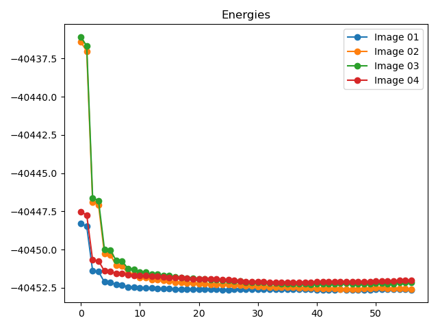
neb计算过程中能量和最大原子受力的变化趋势图

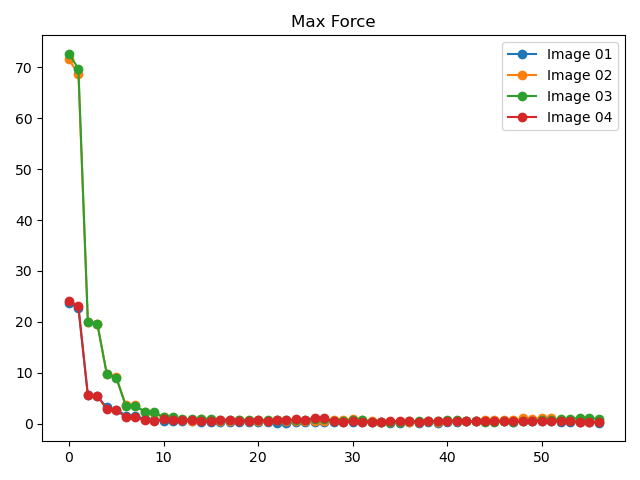
要查看neb计算过程中能量和最大原子受力的变化趋势图，可参考 8neb_energy_force_curves.py ：

# coding:utf-8
from dspawpy.diffusion.nebtools import monitor_force_energy

# Specify the path to the NEB calculation folder; after running, Energies.png and MaxForce.png images will be generated in the specified directory
unfinished_neb_folder = "dspawpy_proj/dspawpy_tests/inputs/supplement/neb_unfinished"
monitor_force_energy(
    directory=unfinished_neb_folder,
    outdir="imgs",  # Output image path
)

将生成能量和受力变化趋势图：

8.9 phonon声子计算数据处理

以MgO体系的声子能带态密度计算得到的 phonon.h5 为例：

如果未安装 phonopy，运行下列脚本时会弹出 no module named 'phonopy' 信息，不影响程序正常运行

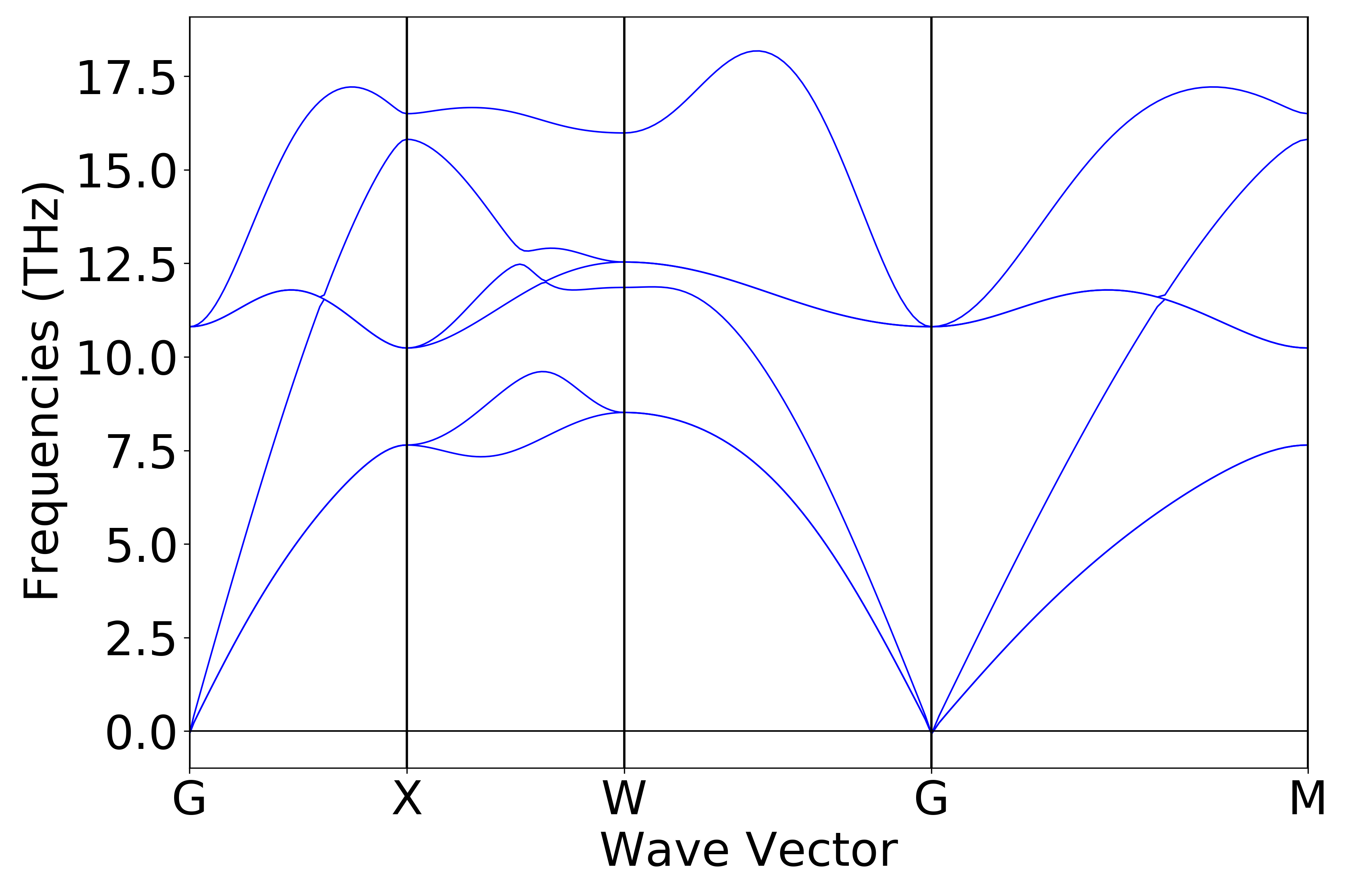
声子能带数据处理

参考 9phonon_bandplot.py ：

# coding:utf-8
import os

from pymatgen.phonon.plotter import PhononBSPlotter

from dspawpy.io.read import get_phonon_band_data

band_data = get_phonon_band_data(
    "dspawpy_proj/dspawpy_tests/inputs/2.16.1/phonon.h5",
)  # Read phonon band structure
bsp = PhononBSPlotter(band_data)
axes_or_plt = bsp.get_plot(ylim=None, units="thz")  # Y-axis range # Units
import matplotlib.pyplot as plt  # noqa: E402

if isinstance(axes_or_plt, plt.Axes):
    fig = axes_or_plt.get_figure()  # version newer than v2023.8.10
elif isinstance(axes_or_plt, tuple):
    fig = axes_or_plt[0].get_figure()
else:
    fig = axes_or_plt.gcf()  # older version pymatgen

filename = "dspawpy_proj/dspawpy_tests/outputs/us/9phonon_bandplot.png"  # File name for the output phonon band plot
os.makedirs(os.path.dirname(os.path.abspath(filename)), exist_ok=True)
fig.savefig(filename, dpi=300)

执行代码可以得到类似以下声子能带曲线：

警告

如果通过SSH连接到远程服务器执行上述脚本，出现QT相关的报错信息，可能是使用的程序（比如MobaXterm等）和QT库不兼容，要么更换程序（例如VSCode或者系统自带的终端命令行），要么请在python脚本第二行开始添加以下代码：

import matplotlib
matplotlib.use('agg')

声子态密度数据处理

参考 9phonon_dosplot.py ：

# coding:utf-8
import os

from pymatgen.phonon.plotter import PhononDosPlotter

from dspawpy.io.read import get_phonon_dos_data

dos = get_phonon_dos_data("dspawpy_proj/dspawpy_tests/inputs/2.16.1/phonon.h5")
dp = PhononDosPlotter(
    stack=False,  # True indicates drawing an area plot
    sigma=None,  # Gaussian blur parameter
)
dp.add_dos(
    label="Phonon", dos=dos
)  # Legend  # The phonon density of states to be plotted
axes_or_plt = dp.get_plot(
    xlim=[0, 20],  # x-axis range
    ylim=None,  # y-axis range
    units="THz",  # Unit
)
import matplotlib.pyplot as plt  # noqa: E402

if isinstance(axes_or_plt, plt.Axes):
    fig = axes_or_plt.get_figure()  # version newer than v2023.8.10
elif isinstance(axes_or_plt, tuple):
    fig = axes_or_plt[0].get_figure()
else:
    fig = axes_or_plt.gcf()  # older version pymatgen

filename = " dspawpy_proj/dspawpy_tests/outputs/us/9phonon_dosplot.png"  # Energy barrier plot output filename
os.makedirs(os.path.dirname(os.path.abspath(filename)), exist_ok=True)
fig.savefig(filename, dpi=300)

执行代码可以得到类似以下声子态密度曲线：

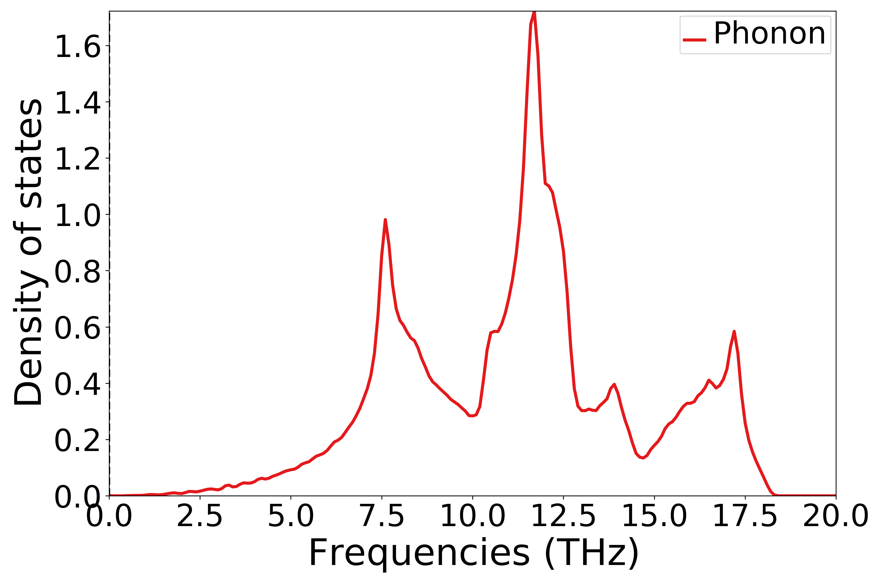
单晶硅声子态密度示意图

警告

如果通过SSH连接到远程服务器执行上述脚本，出现QT相关的报错信息，可能是使用的程序（比如MobaXterm等）和QT库不兼容，要么更换程序（例如VSCode或者系统自带的终端命令行），要么请在python脚本第二行开始添加以下代码：

import matplotlib
matplotlib.use('agg')

声子热力学数据处理

可以参考 9phonon_thermal.py ：

# coding:utf-8
from dspawpy.plot import plot_phonon_thermal

plot_phonon_thermal(
    datafile="dspawpy_proj/dspawpy_tests/inputs/2.26/phonon.h5",  # phonon.h5 data file path
    figname="dspawpy_proj/dspawpy_tests/outputs/us/9phonon.png",  # Output phonon thermodynamics figure filename
    show=False,  # Whether to display the image
)

执行代码可以得到类似以下声子热力学曲线：

单晶硅声子热力学性质示意图

API: get_phonon_band_data(), get_phonon_dos_data(), plot_phonon_thermal()

get_phonon_band_data 函数负责读取声子能带：
dspawpy.io.read.get_phonon_band_data(phonon_band_dir: str, verbose: bool = False)
Reads phonon band data from an h5 or json file and constructs a PhononBandStructureSymmLine object

参数:

phonon_band_dir -- Path to the band structure file, phonon.h5 / phonon.json, or a folder containing these files

返回类型:

PhononBandStructureSymmLine

示例
>>> from dspawpy.io.read import get_phonon_band_data >>> band_data = get_phonon_band_data("dspawpy_proj/dspawpy_tests/inputs/2.16/phonon.h5") # Read phonon band data >>> band_data = get_phonon_band_data("dspawpy_proj/dspawpy_tests/inputs/2.16/phonon.json") # Read phonon band data

get_phonon_dos_data 函数负责读取声子态密度：

dspawpy.io.read.get_phonon_dos_data(phonon_dos_dir: str, verbose: bool = False)

Reads phonon density of states data from an h5 or json file, constructs a PhononDos object

参数:: phonon_dos_dir -- Path to the phonon DOS file, phonon_dos.h5 / phonon_dos.json, or a folder containing these files
返回类型:: PhononDos

示例

>>> from dspawpy.io.read import get_phonon_dos_data
>>> phdos = get_phonon_dos_data(phonon_dos_dir='dspawpy_proj/dspawpy_tests/inputs/2.16.1/phonon.json')
>>> phdos = get_phonon_dos_data(phonon_dos_dir='dspawpy_proj/dspawpy_tests/inputs/2.16.1/phonon.h5')
>>> phdos.frequencies
array([ 0. ,  0.1,  0.2,  0.3,  0.4,  0.5,  0.6,  0.7,  0.8,  0.9,  1. ,
        1.1,  1.2,  1.3,  1.4,  1.5,  1.6,  1.7,  1.8,  1.9,  2. ,  2.1,
        2.2,  2.3,  2.4,  2.5,  2.6,  2.7,  2.8,  2.9,  3. ,  3.1,  3.2,
        3.3,  3.4,  3.5,  3.6,  3.7,  3.8,  3.9,  4. ,  4.1,  4.2,  4.3,
        4.4,  4.5,  4.6,  4.7,  4.8,  4.9,  5. ,  5.1,  5.2,  5.3,  5.4,
        5.5,  5.6,  5.7,  5.8,  5.9,  6. ,  6.1,  6.2,  6.3,  6.4,  6.5,
        6.6,  6.7,  6.8,  6.9,  7. ,  7.1,  7.2,  7.3,  7.4,  7.5,  7.6,
        7.7,  7.8,  7.9,  8. ,  8.1,  8.2,  8.3,  8.4,  8.5,  8.6,  8.7,
        8.8,  8.9,  9. ,  9.1,  9.2,  9.3,  9.4,  9.5,  9.6,  9.7,  9.8,
        9.9, 10. , 10.1, 10.2, 10.3, 10.4, 10.5, 10.6, 10.7, 10.8, 10.9,
       11. , 11.1, 11.2, 11.3, 11.4, 11.5, 11.6, 11.7, 11.8, 11.9, 12. ,
       12.1, 12.2, 12.3, 12.4, 12.5, 12.6, 12.7, 12.8, 12.9, 13. , 13.1,
       13.2, 13.3, 13.4, 13.5, 13.6, 13.7, 13.8, 13.9, 14. , 14.1, 14.2,
       14.3, 14.4, 14.5, 14.6, 14.7, 14.8, 14.9, 15. , 15.1, 15.2, 15.3,
       15.4, 15.5, 15.6, 15.7, 15.8, 15.9, 16. , 16.1, 16.2, 16.3, 16.4,
       16.5, 16.6, 16.7, 16.8, 16.9, 17. , 17.1, 17.2, 17.3, 17.4, 17.5,
       17.6, 17.7, 17.8, 17.9, 18. , 18.1, 18.2, 18.3, 18.4, 18.5, 18.6,
       18.7, 18.8, 18.9, 19. , 19.1, 19.2, 19.3, 19.4, 19.5, 19.6, 19.7,
       19.8, 19.9, 20. ])

plot_phonon_thermal 函数负责绘制声子热力学性质图：
dspawpy.plot.plot_phonon_thermal(datafile: str = 'phonon.h5', figname: str = 'phonon.png', show: bool = True, raw: bool = False, verbose: bool = False)
Task completed for phonon thermodynamic calculations, plot curves of relevant physical quantities versus temperature

phonon.h5/phonon.json -> phonon.png
参数:
datafile -- Path to an h5 or json file or a folder containing any of these files, default 'phonon.h5'

figname -- Filename to save the image

show -- Whether to pop up an interactive interface

raw -- Whether to save the plotting data to rawphonon.csv file
返回:

Image path, default 'phonon.png'

返回类型:

figname
示例
>>> from dspawpy.plot import plot_phonon_thermal >>> plot_phonon_thermal('dspawpy_proj/dspawpy_tests/inputs/2.26/phonon.h5', figname='dspawpy_proj/dspawpy_tests/outputs/doctest/phonon_thermal_h5.png', show=False) >>> plot_phonon_thermal('dspawpy_proj/dspawpy_tests/inputs/2.26/phonon.json', figname='dspawpy_proj/dspawpy_tests/outputs/doctest/phonon_thermal_json.png', show=False, raw=True)

警告

如果通过SSH连接到远程服务器执行上述脚本，出现QT相关的报错信息，可能是使用的程序（比如MobaXterm等）和QT库不兼容，要么更换程序（例如VSCode或者系统自带的终端命令行），要么请在python脚本第二行开始添加以下代码：

import matplotlib
matplotlib.use('agg')

8.10 aimd分子动力学模拟数据处理

以快速入门 \(H_{2}O\) 分子体系分子动力学模拟得到的 aimd.h5 为例：

轨迹文件转换格式为.xyz或.dump

从aimd输出的hdf5文件中读取数据，并生成轨迹文件

生成的.xyz或.dump格式文件，可拖入OVITO观察，通过 Device Studio --> Simulator --> OVITO 打开 OVITO 可视化界面，将xyz文件或dump文件拖入OVITO即可。

参考 10write_aimd_traj.py ：

# coding:utf-8
from dspawpy.io.structure import convert

convert(
    infile="dspawpy_proj/dspawpy_tests/inputs/2.18/aimd.h5",  # Structure to be converted, if in the current path, only the filename can be written
    si=None,  # Filter the configuration number, if not specified, read all by default
    ele=None,  # Filter element symbol, default reads atomic information for all elements
    ai=None,  # Filter atomic indices (starting from 1), default to read all atomic information
    outfile="dspawpy_proj/dspawpy_tests/outputs/us/10aimdTraj.xyz",  # Can also generate .dump files (lower precision), currently only supports orthogonal unit cells
)

执行代码将生成.xyz和.dump格式的轨迹文件，该文件可通过OVITO打开。关于结构文件转化的更多细节，请参考 structure结构转化

知识点：

OVITO 与 dspawpy 都不支持将非正交晶胞的体系保存为dump文件

动力学过程中能量、温度等变化曲线

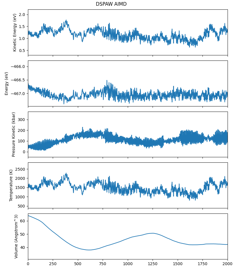
参考 10check_aimd_conv.py ：

# coding:utf-8
from dspawpy.plot import plot_aimd

plot_aimd(
    datafile="dspawpy_proj/dspawpy_tests/inputs/2.18/aimd.h5",  # Data file path
    show=False,  # Whether to pop up the image window
    figname="dspawpy_proj/dspawpy_tests/outputs/us/10aimd.png",  # Output image file name
    flags_str="1 2 3 4 5",  # Select data types
)
# The meaning of flags_str is as follows
# 1. Kinetic energy
# 2. Total Energy
# 3. Pressure
# 4. Temperature
# 5. Volume

执行代码将生成如下组合图：

警告

如果通过SSH连接到远程服务器执行上述脚本，出现QT相关的报错信息，可能是使用的程序（比如MobaXterm等）和QT库不兼容，要么更换程序（例如VSCode或者系统自带的终端命令行），要么请在python脚本第二行开始添加以下代码：

import matplotlib
matplotlib.use('agg')

均方位移（MSD）分析

参考 10aimd_msd.py ：

# coding:utf-8
from dspawpy.analysis.aimdtools import get_lagtime_msd, plot_msd

# If AIMD is not completed in one go, you can assign multiple h5 file paths to the datafile parameter in a list form
lagtime, msd = get_lagtime_msd(
    datafile="dspawpy_proj/dspawpy_tests/inputs/2.18/aimd.h5",  # Data file path
    select="all",  # Default selects all atoms
    msd_type="xyz",  # Default to calculate MSD in the xyz directions
    timestep=None,  # Default reads the timestep from the datafile
)
# Plot the graph using the obtained data and save it
plot_msd(
    lagtime,  # X-axis coordinate
    msd,  # vertical axis
    xlim=None,  # Set the display range of the x-axis
    ylim=None,  # Set the display range of the y-axis
    figname="dspawpy_proj/dspawpy_tests/outputs/us/10MSD.png",  # Output image filename
    show=False,  # Whether to pop up the image window
    ax=None,  # Optional subplot specification
)

执行代码将生成类似如下图片：

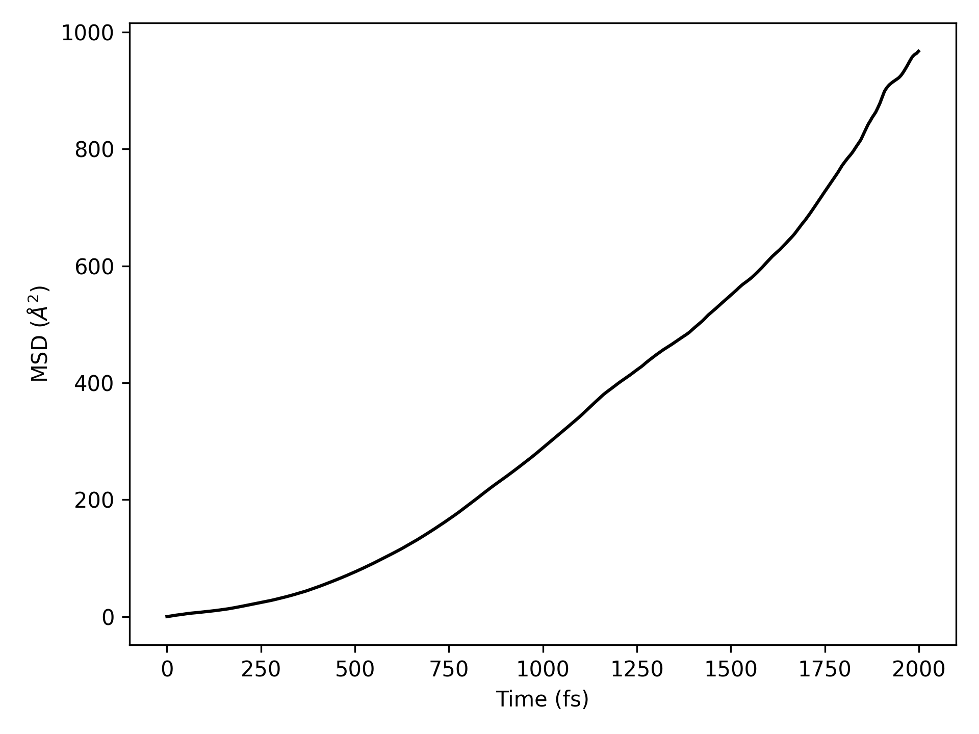
均方位移（MSD）示意图

警告

如果通过SSH连接到远程服务器执行上述脚本，出现QT相关的报错信息，可能是使用的程序（比如MobaXterm等）和QT库不兼容，要么更换程序（例如VSCode或者系统自带的终端命令行），要么请在python脚本第二行开始添加以下代码：

import matplotlib
matplotlib.use('agg')

均方根偏差（RMSD）分析

参考 10aimd_rmsd.py ：

# coding:utf-8
from dspawpy.analysis.aimdtools import get_lagtime_rmsd, plot_rmsd

# If AIMD is not completed in a single run, you can assign multiple paths of h5 files in list form to the datafile parameter
lagtime, rmsd = get_lagtime_rmsd(
    datafile="dspawpy_proj/dspawpy_tests/inputs/2.18/aimd.h5",
    timestep=None,  # Data file path  # Default reads the time step from the datafile
)
plot_rmsd(
    lagtime,  # Horizontal coordinate
    rmsd,  # vertical coordinate
    xlim=None,  # Set the display range of the x-axis
    ylim=None,  # Set the display range of the y-axis
    figname="dspawpy_proj/dspawpy_tests/outputs/us/10RMSD.png",  # Output image filename
    show=False,  # Whether to pop up the image window
    ax=None,  # Optional subplot specification
)

执行代码将生成类似如下图片：

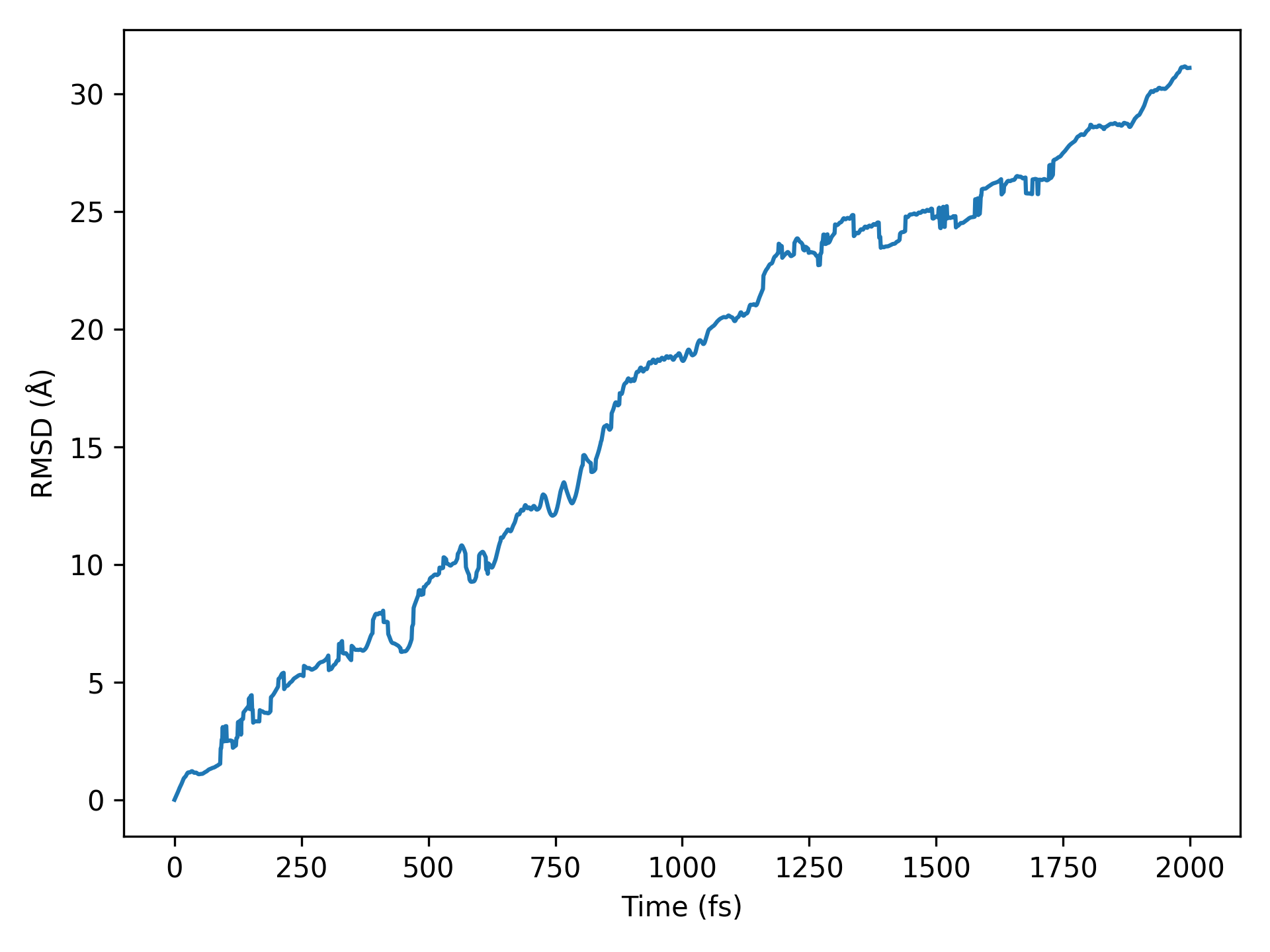
均方根偏差（RMSD）示意图

警告

如果通过SSH连接到远程服务器执行上述脚本，出现QT相关的报错信息，可能是使用的程序（比如MobaXterm等）和QT库不兼容，要么更换程序（例如VSCode或者系统自带的终端命令行），要么请在python脚本第二行开始添加以下代码：

import matplotlib
matplotlib.use('agg')

原子对分布函数或径向分布函数（RDFs）分析

参考 10aimd_rdf.py ：

# coding:utf-8
from dspawpy.analysis.aimdtools import get_rs_rdfs, plot_rdf

# If AIMD is not completed in one go, you can assign multiple h5 file paths to the datafile parameter in the form of a list.
rs, rdfs = get_rs_rdfs(
    datafile="dspawpy_proj/dspawpy_tests/inputs/2.18/aimd.h5",  # Data file path
    ele1="H",  # Central element
    ele2="O",  # Target element
    rmin=0.0,  # Minimum radius
    rmax=10.0,  # Maximum radius
    ngrid=1000,  # Number of grid points
    sigma=0.1,  # sigma value
)
plot_rdf(
    rs,  # x-axis values
    rdfs,  # Vertical coordinate
    "H",  # Central element
    "O",  # Object element
    figname="dspawpy_proj/dspawpy_tests/outputs/us/10RDF.png",  # Image save path
    show=False,  # Whether to pop up the image window
    ax=None,  # Subplot can be specified
)

执行代码将生成类似如下图片：

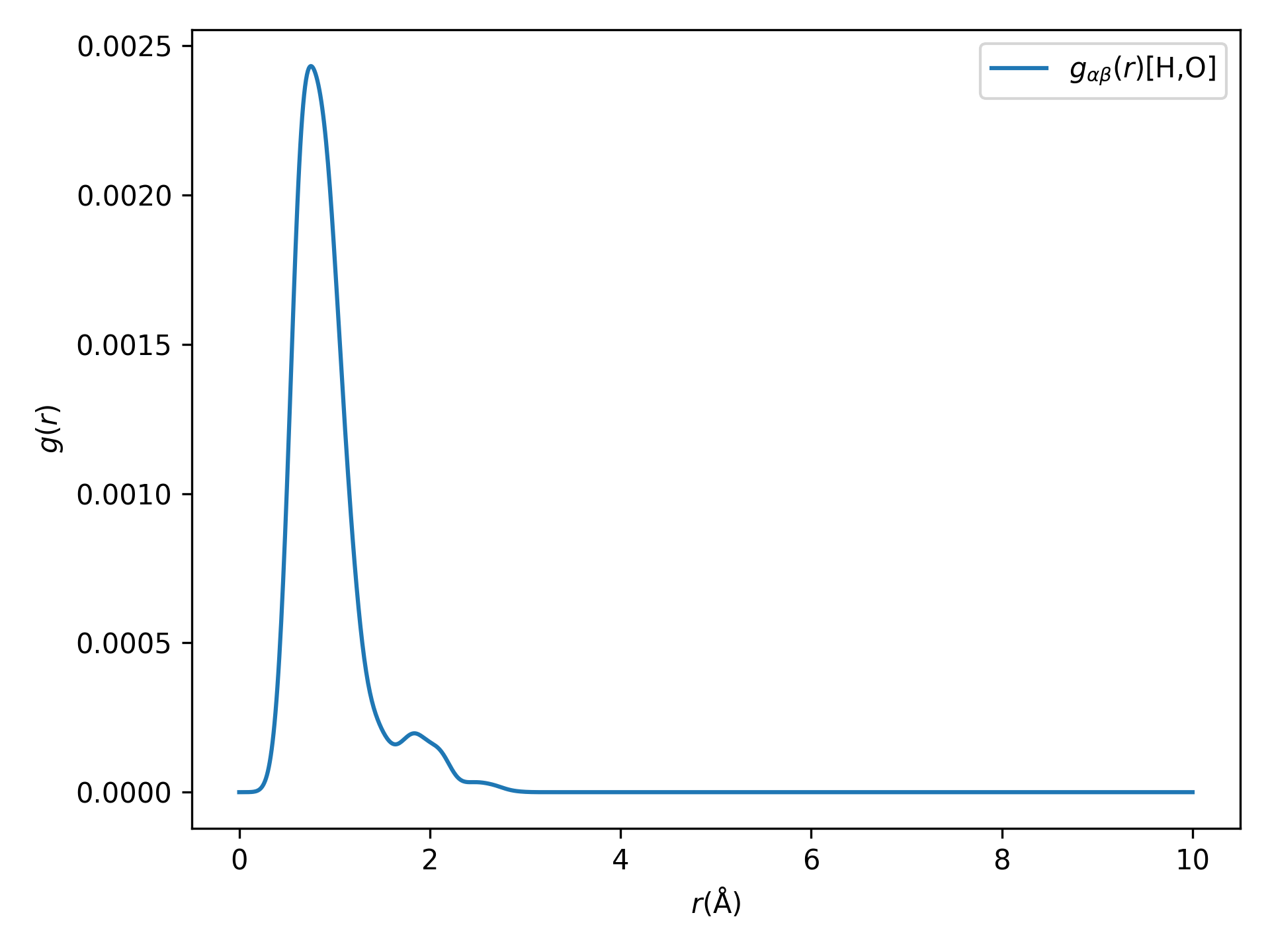
径向分布函数（RDFs）示意图

这部分涉及的统计学计算较复杂，更多细节请参考函数API

警告

如果通过SSH连接到远程服务器执行上述脚本，出现QT相关的报错信息，可能是使用的程序（比如MobaXterm等）和QT库不兼容，要么更换程序（例如VSCode或者系统自带的终端命令行），要么请在python脚本第二行开始添加以下代码：

import matplotlib
matplotlib.use('agg')

8.11 Polarization铁电极化数据处理

以快速入门 \(HfO_{2}\) 体系铁电计算得到的系列 scf.h5 为例：

参考 11Ferri.py ：

# coding:utf-8
from dspawpy.plot import plot_polarization_figure

plot_polarization_figure(
    directory="dspawpy_proj/dspawpy_tests/inputs/2.20",  # Path for iron polarization calculation
    repetition=2,  # Number of times to repeat the data points when plotting
    figname="dspawpy_proj/dspawpy_tests/outputs/us/11pol.png",  # Output polarization figure filename
    show=False,  # Whether to display the polarization figure
)  # --> pol.png

执行代码将生成如下组合图：

12组结构对应极化数值

查看首尾构型的铁电极化数值，可以参考如下：

from dspawpy.plot import plot_polarization_figure

plot_polarization_figure(directory='.', annotation=True, annotation_style=1) # 显示首尾构型的铁电极化数值

执行代码将生成如下组合图：

12组结构对应极化数值（带首尾构型数值）

也可以使用第二种批注样式：

from dspawpy.plot import plot_polarization_figure

plot_polarization_figure(directory='.', annotation=True, annotation_style=2) # 显示首尾构型的铁电极化数值

执行代码将生成如下组合图：

12组结构对应极化数值（带首尾构型数值）

警告

如果通过SSH连接到远程服务器执行上述脚本，出现QT相关的报错信息，可能是使用的程序（比如MobaXterm等）和QT库不兼容，要么更换程序（例如VSCode或者系统自带的终端命令行），要么请在python脚本第二行开始添加以下代码：

import matplotlib
matplotlib.use('agg')

8.12 ZPE零点振动能数据处理

以快速入门 \(CO\) 体系频率计算得到的 frequency.txt 文件为例，计算零点振动能，基于以下公式：

\[ZPE=\sum_{i=1}^{3 N} \frac{h \nu_i}{2}\]

其中， \(\nu_i\) 是简正频率， \(h\) 是普朗克常数（ \(6.626\times10^{-34} J\cdot s\)）， \(N\) 是原子数。

参考 12getZPE.py ：

# coding:utf-8
from dspawpy.io.utils import getZPE

# Import the frequency.txt file obtained from frequency calculation
getZPE(
    fretxt="dspawpy_proj/dspawpy_tests/inputs/2.13/frequency.txt",
)

执行代码结果文件将保存到 ZPE.dat 文件中，文件内容如下：

Data read from D:\quickstart\2.13\frequency.txt
Frequency (meV)
284.840038

--> Zero-point energy,  ZPE (eV): 0.142420019

8.13 TS的热校正能

吸附质的熵变对能量的贡献

计算基于以下公式：

\[\Delta S_{a d s}\left(0 \rightarrow T, P^0\right)=S_{v i b}=\sum_{i=1}^{3 N}\left[\frac{N_{\mathrm{A}} h \nu_i}{T\left(e^{h \nu_i / k_{\mathrm{B}} T}-1\right)}-R \ln \left(1-e^{-h \nu_i / k_{\mathrm{B}} T}\right)\right]\]

其中， \(\Delta S_{a d s}\) 表示吸附质的熵变，根据简谐近似计算。\(S_{v i b}\) 表示振动熵。 \(\nu_i\) 是简正频率，\(N_A\) 是阿伏伽德罗常数（ \(6.022\times10^{23} mol^{-1}\) ）， \(h\) 是普朗克常数（ \(6.626\times10^{-34} J\cdot s\)）， \(k_B\) 是玻尔兹曼常数（ \(1.38\times10^{-23} J\cdot K^{-1}\)）， \(R\) 是理想气体常数（ \(8.314 J\cdot mol^{-1}\cdot K^{-1}\)）， \(T\) 是体系温度，单位 \(K\)。

参考 13getTSads.py ：

# coding:utf-8
from dspawpy.io.utils import getTSads

# Import the frequency.txt file calculated from frequency, temperature can be modified arbitrarily
getTSads(
    fretxt="dspawpy_proj/dspawpy_tests/inputs/2.13/frequency.txt",
    T=298.15,
)

执行代码结果文件将保存到 TS.dat 文件中，文件内容如下：

Data read from D:\quickstart\2.13\frequency.txt
Frequency (THz)
68.873994

--> Entropy contribution,  T*S (eV): 4.7566990201851275e-06

理想气体的熵变对能量的贡献

计算基于如下公式：

\[\begin{split}\begin{aligned} S(T, P) & =S\left(T, P^{\circ}\right)-k_{\mathrm{B}} \ln \frac{P}{P^{\circ}} \\ & =S_{\text {trans }}+S_{\text {rot }}+S_{\text {elec }}+S_{\text {vib }}-k_{\mathrm{B}} \ln \frac{P}{P^{\circ}} \end{aligned}\end{split}\]

其中：

\[S_{\text {trans }}=k_{\mathrm{B}}\left\{\ln \left[\left(\frac{2 \pi M k_{\mathrm{B}} T}{h^2}\right)^{3 / 2} \frac{k_{\mathrm{B}} T}{P^{\circ}}\right]+\frac{5}{2}\right\}\]

\[\begin{split}S_{\mathrm{rot}}= \begin{cases}0 & \text {, monatomic } \\ k_{\mathrm{B}}\left[\ln \left(\frac{8 \pi^2 I k_{\mathrm{B}} T}{\sigma h^2}\right)+1\right] & \text {, linear } \\ k_{\mathrm{B}}\left\{\ln \left[\frac{\sqrt{\pi I_A I_{\mathrm{B}} I_{\mathrm{C}}}}{\sigma}\left(\frac{8 \pi^2 k_B T}{h^2}\right)^{3 / 2}\right]+\frac{3}{2}\right\} & \text {, nonlinear }\end{cases}\end{split}\]

\[S_{\text {elec }}=k_{\mathrm{B}} \ln [2 \times(\text { total spin })+1]\]

\[S_{\text {vib }}=k_{\mathrm{B}} \sum_i^{\text {vib DOF }}\left[\frac{\epsilon_i}{k_{\mathrm{B}} T\left(e^{\epsilon_i / k_{\mathrm{B}} T}-1\right)}-\ln \left(1-e^{-\epsilon_i / k_{\mathrm{B}} T}\right)\right]\]

其中：\(I_A\) 到 \(I_C\) 是非线性分子的三个主惯性矩， \(I\) 是线性分子的简并惯性矩， \(\sigma\) 是分子的对称数。另外，monatomic 表示单原子分子，linear 表示线性分子，nonlinear 表示非线性分子。total spin 是总自旋数。 vib DOF 表示振动自由度。

参考 13getTSgas.py 脚本处理：

# coding:utf-8
from dspawpy.io.utils import getTSgas

# Read elements and coordinates from the calculation result file (json or h5)
TSgas = getTSgas(
    fretxt="dspawpy_proj/dspawpy_tests/inputs/2.13/frequency.txt",
    datafile="dspawpy_proj/dspawpy_tests/inputs/2.13/frequency.h5",
    potentialenergy=-0.0,
    geometry="linear",
    symmetrynumber=1,
    spin=1,
    temperature=298.15,
    pressure=101325.0,
)
print("Entropy contribution, T*S (eV)：", TSgas)

# If only the frequency.txt file is available, the calculation can be completed by manually specifying the elements and coordinates
# TSgas = getTSgas(fretxt='dspawpy_proj/dspawpy_tests/inputs/2.13/frequency.txt', datafile=None, potentialenergy=-0.0, elements=['H', 'H'], geometry='linear', positions=[[0.0, 0.0, 0.0], [0.0, 0.0, 1.0]], symmetrynumber=1, spin=1, temperature=298.15, pressure=101325.0)

8.14 附录

快速下载所有脚本，点击 用户脚本.zip
dspawpy更新日志

8 辅助工具使用教程

8.1 安装与更新

更新 dspawpy

8.2 structure结构转化

8.3 volumetricData数据处理

volumetricData可视化

差分volumetricData可视化

volumetricData面平均

8.4 band能带数据处理

普通能带处理

将能带投影到每一种元素分别作图，数据点大小表示该元素对该轨道的贡献

能带投影到不同元素的不同轨道

将能带投影到不同原子的不同轨道

能带反折叠处理

band-compare能带对比图处理

8.5 dos态密度数据处理

总的态密度

将态密度投影到不同的轨道上

将态密度投影到不同的元素上

将态密度投影到不同原子的不同轨道上

将态密度投影到不同原子的分裂d轨道(t2g, eg)上

d-带中心分析

8.6 bandDos能带和态密度共同显示

将能带和态密度显示在一张图上

将能带和投影态密度显示在一张图上

8.7 optical光学性质数据处理

8.8 neb过渡态计算数据处理

输入文件之生成中间构型

绘制能垒图

neb.iniFin = true/false

neb.iniFin = true

过渡态计算数据处理

观察NEB链

计算构型间距

neb续算

neb计算过程中能量和最大原子受力的变化趋势图

8 LOOP 1:

8.9 phonon声子计算数据处理

声子能带数据处理

声子态密度数据处理

声子热力学数据处理

8.10 aimd分子动力学模拟数据处理

轨迹文件转换格式为.xyz或.dump

动力学过程中能量、温度等变化曲线

均方位移（MSD） 分析

均方根偏差（RMSD） 分析

原子对分布函数或径向分布函数（RDFs） 分析

8.11 Polarization铁电极化数据处理

8.12 ZPE零点振动能数据处理

8.13 TS的热校正能

吸附质的熵变对能量的贡献

理想气体的熵变对能量的贡献

8.14 附录

均方位移（MSD）分析

均方根偏差（RMSD）分析

原子对分布函数或径向分布函数（RDFs）分析